Chapter 6 Enginereing Sustainability: Evapotranspiraiton

Chapter 6 Enginereing Sustainability: Evapotranspiraiton#

Introduction: Evapotranspiration
Simulation: Evapotranspiration
Self-Assessment

1. Introduction#

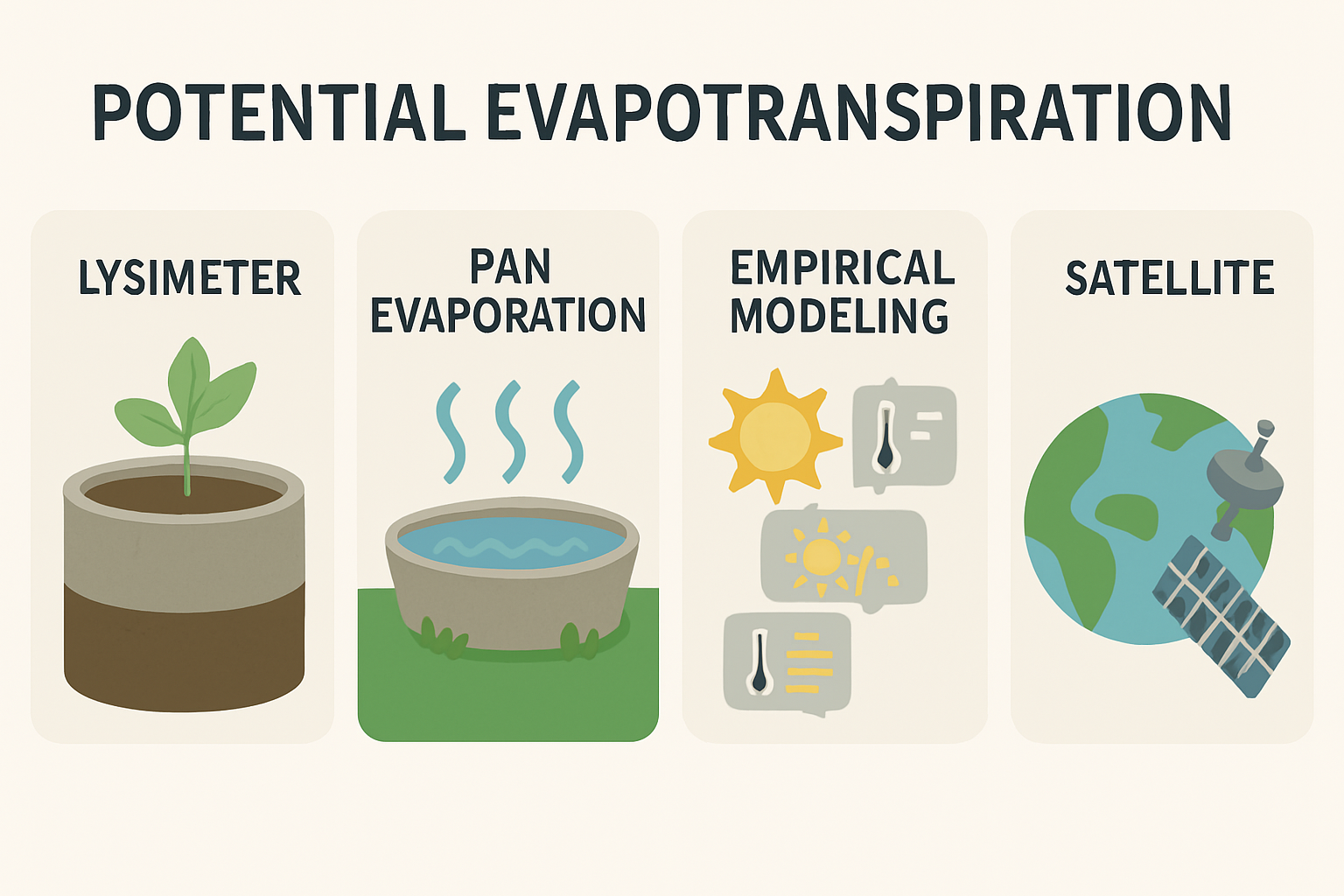
Descriptive alt text for accessibility — Fig. 39 **Figure 6.5 **: Potential Evpotranspiration#

💧 Evapotranspiration (ET): Definition, Importance, and Measurement#

🧭 Definition#

Evapotranspiration (ET) is the combined process of:

Evaporation: Water loss from soil, water bodies, and surfaces to the atmosphere
Transpiration: Water movement from plant roots to leaves and release as vapor through stomata

Together, ET represents the total water flux from land to atmosphere, and is a key component of the hydrological cycle.

🌍 Role in the Hydrological Cycle#

ET returns 60–75% of terrestrial precipitation back to the atmosphere
Drives soil moisture depletion, plant water use, and climate feedbacks
Influences groundwater recharge, runoff, and crop water demand

🌱 Importance in Sustainable Development#

🛰️ ET is a proxy for irrigation demand and crop water use
🌾 Helps optimize agricultural water management
🌡️ Critical for drought monitoring, climate modeling, and ecosystem health
📈 Supports SDG 6 (Clean Water) and SDG 13 (Climate Action)

🧪 How ET Is Measured#

🔬 Direct Methods#

Method	Description
Lysimeter	Measures weight change of soil-plant system to estimate water loss
Pan Evaporation	Uses open water pans to estimate potential evaporation
Eddy Covariance	Measures vapor flux using wind and humidity sensors

⚠️ Direct methods are accurate but expensive and limited in spatial coverage.

🧠 Modeling ET with Meteorological and Satellite Data#

📊 Meteorological Models#

Use solar radiation, temperature, humidity, wind
Apply equations like Penman-Monteith, Hargreaves, or Blaney-Criddle

🛰️ Satellite-Based Models#

Use thermal and optical imagery + weather data
Estimate actual ET over large areas with high resolution

🚀 OPENET: Satellite-Based ET Estimation#

🔍 What Is OPENET?#

A NASA-led platform providing field-scale ET data across the western U.S.
Uses Landsat imagery, meteorological grids, and ensemble modeling

🧮 Algorithms Used#

Model	Approach	Reference
METRIC	Surface energy balance	Allen et al. (2007)
SEBAL	Energy balance with calibration	Bastiaanssen et al. (1998)
PT-JPL	Priestley-Taylor with constraints	Fisher et al. (2008)
SSEBop	Simplified energy balance	Senay et al. (2013)
SIMS	Crop coefficient from NDVI	Melton et al. (2012)
DisALEXI	Two-source energy balance	Anderson et al. (2018)

📈 Inputs#

Landsat thermal and optical data
Gridded weather datasets (e.g., gridMET, PRISM)
Crop type, land use, soil data

📌 Features#

30m resolution ET maps
Daily, monthly, annual ET estimates
Ensemble averaging across models
Used by water agencies for irrigation planning, water rights, and conservation

🔗 OPENET Methodologies

🧠 Summary Insight#

Evapotranspiration is a critical link between land, vegetation, and atmosphere. While direct measurement is costly, modern satellite platforms like OPENET enable scalable, accurate, and timely ET estimation—empowering sustainable water management and climate resilience.

Reference#

[] developed a scalable monthly ET model using FAO-56 reference ET (ETo), precipitation (P), and leaf area index (LAI), explaining ~85% of ET variability across 13 ecosystems. They emphasized the value of remote sensing and weather data, noting that wet forests often exceed ETo while arid regions fall below it. [] evaluated 127 potential evapotranspiration (PET) models across Mediterranean urban green sites, classifying them into temperature-, radiation-, mass-transfer, and combination-based methods. Temperature-based models performed best in data-scarce environments, with 22 models showing <10% deviation from the FAO-56 Penman-Monteith benchmark. They stressed the need for site-specific calibration. [Weiß and Menzel, 2008] reviewed empirical PET models and their meteorological drivers, highlighting Hargreaves-Samani (temperature), Priestley-Taylor (radiation), and Penman-Monteith (full suite).

🌿 Theoretical Background: Potential Evapotranspiration (PET) Models#

Evapotranspiration (ET) represents the combined loss of water from soil evaporation and plant transpiration. Estimating potential evapotranspiration (PET) is essential for hydrological modeling, irrigation planning, and climate impact assessment. The models below vary in complexity, data requirements, and physical assumptions.

🔀 Mixed-Method Models#

1. Penman (1948)#

Combines energy balance and aerodynamic principles. Requires temperature, radiation, humidity, and wind speed.

Equation: $$ ET = \frac{\Delta R_n + \gamma \frac{900}{T + 273} u (e_s - e_a)}{\Delta + \gamma (1 + 0.34u)} $$

$( R_n $): net radiation (MJ/m²/day)
$( T $): mean air temperature (°C)
$( u $): wind speed (m/s)
$( e_s $), $( e_a $): saturation and actual vapor pressure (kPa)
$( \Delta $): slope of vapor pressure curve
$( \gamma $): psychrometric constant

2. Turc (1961)#

Empirical model using temperature, solar radiation, and relative humidity.

Equation: $$ ET = \frac{0.013 \cdot (T / (T + 15)) \cdot (Rs + 50)}{\sqrt{RH / 100}} $$

$( T $): mean temperature (°C)
$( Rs $): solar radiation (MJ/m²/day)
$( RH $): relative humidity (%)

🌞 Radiation-Based Models#

3. Priestley-Taylor (1972)#

Simplified energy balance model assuming minimal aerodynamic influence.

Equation: $$ ET = \alpha \cdot \frac{\Delta}{\Delta + \gamma} \cdot R_n $$

$( \alpha $): empirical coefficient (~1.26)
$( R_n $): net radiation
$( \Delta $), $( \gamma $): as above

4. Makkink (1957)#

Uses temperature and radiation, calibrated for temperate climates.

Equation: $$ ET = 0.61 \cdot \frac{\Delta}{\Delta + \gamma} \cdot Rs $$

$( Rs $): solar radiation
$( \Delta $), $( \gamma $): as above

🌡️ Temperature-Based Models#

5. Thornthwaite (1948)#

Empirical model based solely on temperature and latitude.

Equation: $$ ET = 16 \cdot \left(\frac{10T}{I}\right)^a $$

$( T $): mean monthly temperature (°C)
$( I $): annual heat index
$( a $): empirical exponent based on $( I $)

6. Hamon (1963)#

Estimates ET using temperature and day length.

Equation: $$ ET = 0.1651 \cdot D \cdot \frac{e_s}{T + 273.2} $$

$( D $): day length (hours)
$( e_s $): saturation vapor pressure

📉 Temperature-Radiation Hybrid Models#

7. Hargreaves-Samani (1985)#

Uses temperature range and extraterrestrial radiation.

Equation: $$ ET = 0.0023 \cdot (T_{mean} + 17.8) \cdot (T_{max} - T_{min})^{0.5} \cdot R_a $$

$( R_a $): extraterrestrial radiation
$( T_{mean} $), $( T_{max} $), $( T_{min} $): temperatures

🧠 Simplified Empirical Model#

8. Oudin (2005)#

Minimalist model using temperature and latitude.

Equation: $$ ET = \frac{Rs}{100} \cdot \left(\frac{T + 5}{100}\right) $$

Often reformulated using temperature and latitude-based radiation estimates.

🧪 Model Selection Considerations#

Model	Inputs Required	Complexity	Best Use Case
Penman	T, RH, Rs, wind	High	Detailed hydrological modeling
Priestley-Taylor	T, Rs	Medium	Energy-dominated environments
Hargreaves-Samani	T_max, T_min, latitude	Medium	Data-sparse regions
Thornthwaite	T, latitude	Low	Long-term climate analysis
Turc	T, Rs, RH	Medium	Mediterranean climates
Makkink	T, Rs	Medium	Temperate zones
Hamon	T, latitude	Low	Simpler water balance models
Oudin	T, latitude	Very Low	Quick screening or large datasets

2. Simulation#

import pandas as pd
import matplotlib.pyplot as plt
import pyet

# 📥 Load and preprocess data

# data = pd.read_csv("WR_alexandria.csv", parse_dates=True, index_col="date")
# data = pd.read_csv("WR_alexandria.csv", parse_dates=True, index_col="date")

# # 🌤️ Meteorological inputs
# meteo = pd.DataFrame({
#     "tmax": data["tmax"],
#     "tmin": data["tmin"],
#     "rain": data["rain"],
#     "umax": data["maxu2"] * 0.447,  # convert to m/s
#     "u": data["u2"] * 0.447,
#     "rhmax": data["rhmax"] / 100,
#     "rhmin": data["rhmin"] / 100,
#     "sol": data["solar"],
#     "tsmax": data["tsmax"],
#     "tsmin": data["tsmin"]
# })


# 📥 Read the tab-separated file
#df = pd.read_csv('WR_Alexandria.csv', parse_dates = True, parse_dates=['date'])
#df = pd.read_csv('WR_Alexandria.csv', sep='\t', parse_dates=['date'])

df = pd.read_csv('WR_Alexandria.csv', sep=',', parse_dates=['date'])
#with open('WR_Alexandria.csv', 'r') as f:
#    print(f.readline())
#date,tmax,tmin,rain,maxu2,u2,u2dir,rhmax,rhmin,solar,tsmax,tsmin

# 🧼 Clean and convert numeric columns
numeric_cols = df.columns.drop('date')  # all except date

for col in numeric_cols:
    # Strip whitespace, convert to numeric, coerce errors to NaN
    df[col] = pd.to_numeric(df[col], errors='coerce')

# 🧹 Optional: Handle missing values (if any)
df.fillna(method='ffill', inplace=True)  # forward fill
# Or: df.dropna(inplace=True)

# ✅ Display summary
print(df)
#print("\nData types:\n", df.dtypes)

# 🌍 Site parameters
lat = 39 * 3.1416 / 180  # radians
elevation = 10  # meters

# 🌡️ Derived variables
tmean = (data["tmax"] + data["tmin"]) / 2.0
rh = (data["rhmax"] + data["rhmin"]) / 2.0
sol = data["solar"]
tmax = data["tmax"]
tmin = data["tmin"]
u = data["u2"] * 0.447  # wind speed in m/s
#print(tmean)
#plt.plot(u)
# 🧮 Evapotranspiration Models

# 🔀 Mixed-methods
#et_penman = pyet.penman(tmean, u, rs=sol, elevation=elevation, lat=lat, tmax=tmax, tmin=tmin, rh=rh)
et_oudin = pyet.oudin(tmean, lat)
#et_makkink = pyet.makkink(tmean, rs=sol, elevation=elevation)
et_turc = pyet.turc(tmean, rs=sol, rh=rh)

# 🌞 Radiation-based
#et_priestley_taylor = pyet.priestley_taylor(tmean, rs=sol, elevation=elevation)
#et_hargreaves = pyet.hargreaves(tmean, tmax, tmin, lat)

# 🌡️ Temperature-based
#et_thornthwaite = pyet.thornthwaite(tmean, lat)
#et_hamon = pyet.hamon(tmean, lat)

# 📊 Plot comparison
plt.figure(figsize=(12, 6))
et_penman.plot(label="Penman", color="blue")
et_priestley_taylor.plot(label="Priestley-Taylor", color="green")
et_hargreaves.plot(label="Hargreaves-Samani", color="orange")
et_thornthwaite.plot(label="Thornthwaite", color="purple")
et_hamon.plot(label="Hamon", color="brown")
et_oudin.plot(label="Oudin", color="gray")
et_makkink.plot(label="Makkink", color="teal")
et_turc.plot(label="Turc", color="red")

plt.title("Evapotranspiration Estimates — Multiple Models")
plt.ylabel("ET (mm/day)")
plt.xlabel("Date")
plt.grid(True)
plt.legend()
plt.tight_layout()
plt.show()

---------------------------------------------------------------------------
FileNotFoundError                         Traceback (most recent call last)
Cell In[3], line 29
import pyet
# 📥 Load and preprocess data

# data = pd.read_csv("WR_alexandria.csv", parse_dates=True, index_col="date")
   (...)
#df = pd.read_csv('WR_Alexandria.csv', parse_dates = True, parse_dates=['date'])
#df = pd.read_csv('WR_Alexandria.csv', sep='\t', parse_dates=['date'])
---> 29 df = pd.read_csv('WR_Alexandria.csv', sep=',', parse_dates=['date'])
#with open('WR_Alexandria.csv', 'r') as f:
#    print(f.readline())
#date,tmax,tmin,rain,maxu2,u2,u2dir,rhmax,rhmin,solar,tsmax,tsmin

# 🧼 Clean and convert numeric columns
numeric_cols = df.columns.drop('date')  # all except date

File ~\anaconda3\Lib\site-packages\pandas\io\parsers\readers.py:1026, in read_csv(filepath_or_buffer, sep, delimiter, header, names, index_col, usecols, dtype, engine, converters, true_values, false_values, skipinitialspace, skiprows, skipfooter, nrows, na_values, keep_default_na, na_filter, verbose, skip_blank_lines, parse_dates, infer_datetime_format, keep_date_col, date_parser, date_format, dayfirst, cache_dates, iterator, chunksize, compression, thousands, decimal, lineterminator, quotechar, quoting, doublequote, escapechar, comment, encoding, encoding_errors, dialect, on_bad_lines, delim_whitespace, low_memory, memory_map, float_precision, storage_options, dtype_backend)
kwds_defaults = _refine_defaults_read(
   dialect,
   delimiter,
   (...)
   dtype_backend=dtype_backend,
)
kwds.update(kwds_defaults)
-> 1026 return _read(filepath_or_buffer, kwds)

File ~\anaconda3\Lib\site-packages\pandas\io\parsers\readers.py:620, in _read(filepath_or_buffer, kwds)
_validate_names(kwds.get("names", None))
# Create the parser.
--> 620 parser = TextFileReader(filepath_or_buffer, **kwds)
if chunksize or iterator:
   return parser

File ~\anaconda3\Lib\site-packages\pandas\io\parsers\readers.py:1620, in TextFileReader.__init__(self, f, engine, **kwds)
   self.options["has_index_names"] = kwds["has_index_names"]
self.handles: IOHandles | None = None
-> 1620 self._engine = self._make_engine(f, self.engine)

File ~\anaconda3\Lib\site-packages\pandas\io\parsers\readers.py:1880, in TextFileReader._make_engine(self, f, engine)
   if "b" not in mode:
       mode += "b"
-> 1880 self.handles = get_handle(
   f,
   mode,
   encoding=self.options.get("encoding", None),
   compression=self.options.get("compression", None),
   memory_map=self.options.get("memory_map", False),
   is_text=is_text,
   errors=self.options.get("encoding_errors", "strict"),
   storage_options=self.options.get("storage_options", None),
)
assert self.handles is not None
f = self.handles.handle

File ~\anaconda3\Lib\site-packages\pandas\io\common.py:873, in get_handle(path_or_buf, mode, encoding, compression, memory_map, is_text, errors, storage_options)
elif isinstance(handle, str):
   # Check whether the filename is to be opened in binary mode.
   # Binary mode does not support 'encoding' and 'newline'.
   if ioargs.encoding and "b" not in ioargs.mode:
       # Encoding
--> 873         handle = open(
           handle,
           ioargs.mode,
           encoding=ioargs.encoding,
           errors=errors,
           newline="",
       )
   else:
       # Binary mode
       handle = open(handle, ioargs.mode)

FileNotFoundError: [Errno 2] No such file or directory: 'WR_Alexandria.csv'

3. Self-Assessment#

🌿 Reflective, Conceptual, and Quiz Questions: Potential Evapotranspiration (PET) Models#

📘 Conceptual Questions#

These questions explore the physical principles, assumptions, and structure of the PET models.

General Concepts#

What is the difference between actual evapotranspiration (ET) and potential evapotranspiration (PET)?
Why is PET a critical variable in hydrology, agriculture, and climate modeling?
How do meteorological inputs like temperature, radiation, humidity, and wind influence PET?

Model Structure#

What distinguishes mixed-method models (e.g., Penman) from purely empirical or temperature-based models?
Why do radiation-based models often assume minimal aerodynamic influence?
How does latitude affect temperature-based models like Thornthwaite and Hamon?

Data Requirements#

Which models are best suited for data-scarce environments, and why?
How does the complexity of a model relate to its input requirements and accuracy?
What are the trade-offs between using a simplified model like Oudin versus a physically-based model like Penman?

🔍 Reflective Questions#

These questions encourage critical thinking and application to real-world modeling decisions.

If you were modeling PET for a remote watershed with limited data, which model would you choose and why?
How might climate change (e.g., increased temperature, altered radiation patterns) affect the reliability of temperature-based PET models?
What are the implications of overestimating PET in irrigation planning or drought forecasting?
How could you validate the performance of different PET models using observed ET data?
In what scenarios might a medium-complexity model like Hargreaves-Samani outperform a high-complexity model like Penman?

❓ Quiz Questions#

Multiple Choice#

Which PET model requires the most meteorological inputs?
A. Oudin
B. Hamon
C. Penman
D. Thornthwaite
Answer: C
Which model is most appropriate for long-term climate analysis using only temperature and latitude?
A. Priestley-Taylor
B. Thornthwaite
C. Turc
D. Makkink
Answer: B
In the Hargreaves-Samani model, which variable represents extraterrestrial radiation?
A. ( R_s )
B. ( R_n )
C. ( R_a )
D. ( e_s )
Answer: C

True/False#

The Priestley-Taylor model assumes minimal influence from wind and humidity.
Answer: True
The Oudin model requires solar radiation and wind speed as inputs.
Answer: False
All PET models estimate actual evapotranspiration under field conditions.
Answer: False

Short Answer#

Explain why the Penman model is considered physically rigorous.
Answer: It integrates both energy balance and aerodynamic components, accounting for radiation, temperature, humidity, and wind speed.
What are the limitations of using temperature-only models like Thornthwaite in arid regions?
Answer: They may underestimate PET due to lack of radiation and humidity inputs, which are critical in dry climates.