
Chapter 2 Hydrology: Rainfall frequency analysis#
1. Introduction#
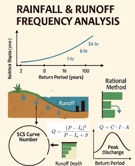
Fig. 2 ** Figure 2.1**: Rainfall/Runoff Frequency Analysis.#
Rainfall frequency analysis#
Rainfall frequency analysis helps engineers and planners estimate how often specific rainfall events are likely to occur, such as a “10-year storm.” These statistics are essential for designing drainage infrastructure, managing flood risks, and sizing stormwater systems.
The SCS Curve Number (CN) method is a widely used empirical approach that estimates surface runoff from rainfall based on land use, soil type, and hydrologic conditions. When paired with frequency-based rainfall inputs from NOAA Atlas 14, it enables realistic modeling of watershed response across various return periods and storm durations.
This learning module is designed to reinforce your understanding of:
How rainfall depth varies with return period across different durations
The role of CN in shaping runoff response
The interplay between frequency-based rainfall and runoff generation
Explore the questions and quiz below to apply these concepts and reflect on their real-world implications.
NOAA Rainfall Frequency & SCS Runoff Estimation Tool#
This script visualizes rainfall depth-frequency data from a NOAA Atlas 14 CSV file and estimates runoff using the SCS Curve Number method.
Rainfall Frequency & Runoff Estimation Toolkit#
This interactive tool uses precipitation frequency data (from NOAA Atlas 14) to estimate surface runoff using two common hydrologic methods:
SCS Curve Number (CN) Method
Rational Method
It enables side-by-side exploration of how different design storms (e.g., 2-year, 25-year) and watershed conditions affect runoff depth or peak discharge.
Methods Overview#
SCS Curve Number (CN) Method#
The SCS method [United States Department of Agriculture, Natural Resources Conservation Service, 2021] estimates runoff volume based on total storm depth and watershed characteristics.
Where:
\(( Q \)): runoff depth (mm)
\(( P \)): rainfall depth (mm)
\(( CN \)): Curve Number (dimensionless, 30–100)
\(( S \)): maximum potential retention (mm)
\(( I_a \)): initial abstraction (mm)
Use this method when estimating total runoff depth from a storm event for a given land cover and soil condition.
Rational Method#
The Rational formula [of Transportation, 2020] estimates peak runoff rate based on rainfall intensity and watershed area.
Where:
\(( Q \)): peak runoff (m³/s)
\(( C \)): runoff coefficient (depends on land use)
\(( I \)): rainfall intensity (mm/hr)
\(( A \)): drainage area (hectares)
This method is most appropriate for small urban catchments with short time of concentration, where peak flow is the design priority.
Interactive Controls#
You can explore:
Storm durations (e.g., 1-hr, 6-hr, 24-hr) from NOAA frequency tables
Return periods (e.g., 2-year, 100-year)
Runoff parameters:
Curve Number (30–100) for the SCS method
Runoff coefficient \(( C \)) and drainage area (ha) for the Rational method
Outputs#
Rainfall depth or intensity vs. return period
Runoff (depth or peak flow) vs. return period
Tabular summaries comparing inputs and outputs
Learning Outcomes#
Understand how watershed characteristics influence runoff response
Compare SCS and Rational methods under varying storm scenarios
Visualize how design rainfall translates to discharge for infrastructure sizing
Key Features#
Automatic CSV Processing:
Loads NOAA rainfall frequency data (e.g., “All_Depth_English_PDS.csv”)
Extracts durations and return periods (e.g., 2-year, 10-year storms)
Converts rainfall depths from inches to mm for SCS runoff estimation
** Rainfall Frequency Visualization:**
Static plot of rainfall depth vs. return period across multiple durations
** SCS Runoff Calculation:**
Implements standard SCS runoff formula:
Curve Number (CN) adjustable via slider (range: 30–100)
Rational runoff calculation
** Interactive Analysis:**
Interactive plot comparing rainfall depth and resulting runoff for selected storm duration
Tabular output showing return period vs. rainfall and runoff
Applications#
Hydrologic modeling
Stormwater system design
Educational demonstrations of rainfall-runoff relationships 💡 Use cases include urban drainage design, floodplain analysis, and stormwater infrastructure planning.
Foundational Literature#
[United States Department of Agriculture, Natural Resources Conservation Service, 2021],[of Transportation, 2020] provide foundational guidance for rainfall frequency analysis and runoff estimation using the SCS (NRCS) Curve Number method and the Rational method, respectively. These methods help engineers and planners estimate how often specific rainfall events—like a “10-year storm”—are likely to occur, which is critical for designing drainage infrastructure, managing flood risks, and sizing stormwater systems. [United States Department of Agriculture, Natural Resources Conservation Service, 2021] outlines the Curve Number (CN) method, which estimates runoff volume based on land use, soil type, and antecedent moisture conditions. It includes updated rainfall distributions and hydrograph generation techniques for spatio-temporal runoff modeling. {cite:p}`TxDOT_Rational provides procedures for estimating peak discharge using rainfall intensity-duration-frequency (IDF) curves and time of concentration. It is widely used for small urban watersheds and includes updated IDF coefficients based on NOAA Atlas 14 data. Together, these resources form the backbone of practical hydrologic design in the U.S., especially for stormwater and flood control applications.
2. Simulation#
import pandas as pd
from io import StringIO

data = """\
Duration    1   2   5   10  25  50  100 200 500 1000
5-min       0.543   0.622   0.754   0.864   1.02    1.14    1.26    1.39    1.55    1.68
10-min      0.795   0.911   1.1     1.26    1.49    1.67    1.85    2.03    2.28    2.46
15-min      0.969   1.11    1.35    1.54    1.82    2.03    2.25    2.48    2.78    3
30-min      1.49    1.73    2.11    2.43    2.88    3.23    3.58    3.94    4.42    4.79
60-min      2.02    2.32    2.84    3.32    4.02    4.61    5.24    5.92    6.87    7.64
2-hr        2.55    2.91    3.58    4.20    5.16    6       6.9     7.89    9.32    10.5
3-hr        2.86    3.26    4.02    4.77    5.96    7.01    8.18    9.48    11.4    13
6-hr        3.38    3.90    4.92    5.92    7.5     8.9     10.5    12.2    14.7    16.8
12-hr       3.90    4.65    6.01    7.28    9.21    10.9    12.6    14.6    17.4    19.7
24-hr       4.58    5.46    7.02    8.44    10.6    12.4    14.3    16.4    19.3    21.7
2-day       5.42    6.26    7.80    9.24    11.5    13.4    15.4    17.7    20.9    23.6
3-day       5.82    6.73    8.38    9.91    12.3    14.3    16.4    18.8    22.2    25
4-day       6.14    7.11    8.88    10.5    13.0    15.1    17.4    19.8    23.4    26.2
7-day       7.07    8.16    10.1    11.9    14.6    16.9    19.4    22.1    25.9    29
10-day      7.99    9.14    11.2    13.1    16.0    18.4    20.9    23.7    27.7    30.9
20-day      10.7    12.1    14.5    16.6    19.7    22.2    24.8    27.6    31.5    34.6
30-day      13.0    14.6    17.4    19.7    23.0    25.6    28.2    31.0    34.8    37.7
45-day      16.0    17.9    21.2    23.8    27.5    30.2    33.0    35.8    39.4    42.1
60-day      18.5    20.8    24.5    27.5    31.5    34.5    37.4    40.2    43.8    46.4
"""

df = pd.read_csv(StringIO(data), delim_whitespace=True)
df.head()
C:\Users\satis\AppData\Local\Temp\ipykernel_15428\3816546494.py:27: FutureWarning: The 'delim_whitespace' keyword in pd.read_csv is deprecated and will be removed in a future version. Use ``sep='\s+'`` instead
  df = pd.read_csv(StringIO(data), delim_whitespace=True)
| Duration | 1 | 2 | 5 | 10 | 25 | 50 | 100 | 200 | 500 | 1000 | |
|---|---|---|---|---|---|---|---|---|---|---|---|
| 0 | 5-min | 0.543 | 0.622 | 0.754 | 0.864 | 1.02 | 1.14 | 1.26 | 1.39 | 1.55 | 1.68 |
| 1 | 10-min | 0.795 | 0.911 | 1.100 | 1.260 | 1.49 | 1.67 | 1.85 | 2.03 | 2.28 | 2.46 |
| 2 | 15-min | 0.969 | 1.110 | 1.350 | 1.540 | 1.82 | 2.03 | 2.25 | 2.48 | 2.78 | 3.00 |
| 3 | 30-min | 1.490 | 1.730 | 2.110 | 2.430 | 2.88 | 3.23 | 3.58 | 3.94 | 4.42 | 4.79 |
| 4 | 60-min | 2.020 | 2.320 | 2.840 | 3.320 | 4.02 | 4.61 | 5.24 | 5.92 | 6.87 | 7.64 |
import pandas as pd
import matplotlib.pyplot as plt
from ipywidgets import interact, IntSlider, FloatSlider, Dropdown
from IPython.display import display, Markdown

# --- Load NOAA CSV File ---
# csv_file = "All_Depth_English_PDS.csv"  # Replace with your actual file path
# df = pd.read_csv(csv_file)

if 'Duration' not in df.columns:
    raise ValueError("CSV does not contain a 'Duration' column.")

df.set_index('Duration', inplace=True)

# Extract numeric return period columns
valid_columns = [col for col in df.columns if any(char.isdigit() for char in col)]
df_filtered = df[valid_columns]

# Convert columns like "2-year" → 2
def extract_return_period(label):
    try:
        return int(label.split('-')[0])
    except:
        return None

df_T = df_filtered.T
df_T.index = df_T.index.map(extract_return_period)
df_T = df_T.dropna().sort_index()
df_T.columns.name = None

# --- SCS Curve Number Runoff Function ---
def scs_runoff(P, CN):
    if CN <= 0 or CN > 100:
        return None
    S = (25400 / CN) - 254  # mm
    Ia = 0.2 * S
    if P <= Ia:
        return 0.0
    else:
        Q = ((P - Ia) ** 2) / (P - Ia + S)
        return round(Q, 2)

# --- Rational Method Runoff Function ---
def rational_runoff(C, I, A):
    if not (0 < C <= 1):
        return None
    Q = C * I * A * 0.00278  # I in mm/hr, A in ha → Q in m³/s
    return round(Q, 2)

# --- Plotting Function ---
def plot_runoff(method, duration, CN=75, C=0.6, A=10):
    if duration not in df_T.columns:
        print(f"❌ Duration '{duration}' not available.")
        return

    intensity_in = df_T[duration]  # inches
    intensity_mm = intensity_in * 25.4  # mm total depth

    fig, ax = plt.subplots(figsize=(8, 5))

    if method == "SCS Curve Number":
        P = intensity_mm
        runoff = P.apply(lambda p: scs_runoff(p, CN))
        ax.plot(P.index, P.values, 'o-', label="Rainfall Depth (mm)", color='dodgerblue')
        ax.plot(runoff.index, runoff.values, 's-', label="SCS Runoff Depth (mm)", color='orangered')
        ax.set_ylabel("Depth (mm)")
        display(Markdown(f"### 📊 SCS Runoff Summary for {duration} (CN = {CN})"))
        display(pd.DataFrame({'Rainfall (mm)': P.round(1), 'Runoff (mm)': runoff}, index=P.index))

    elif method == "Rational Method":
        # Assume depth ≈ intensity for short duration (simplification)
        I = (intensity_mm / (1 if 'hr' in duration else 1))  # mm/hr
        Q = I.apply(lambda i: rational_runoff(C, i, A))
        ax.plot(I.index, I.values, 'o-', label="Rainfall Intensity (mm/hr)", color='steelblue')
        ax.plot(Q.index, Q.values, 's-', label="Peak Runoff Q (m³/s)", color='darkgreen')
        ax.set_ylabel("Value")
        display(Markdown(f"### ⚡ Rational Method Runoff for {duration} (C = {C}, A = {A} ha)"))
        display(pd.DataFrame({'Intensity (mm/hr)': I.round(1), 'Peak Q (m³/s)': Q}, index=I.index))

    ax.set_title(f"{method} – {duration} Storm")
    ax.set_xlabel("Return Period (years)")
    ax.grid(True, linestyle="--", alpha=0.5)
    ax.legend()
    plt.tight_layout()
    plt.show()

# --- Launch Interactive Tool ---
available_durations = df_T.columns.tolist()

interact(
    plot_runoff,
    method=Dropdown(options=["SCS Curve Number", "Rational Method"], value="SCS Curve Number"),
    duration=Dropdown(options=available_durations),
    CN=IntSlider(value=75, min=30, max=100, step=1, description="Curve Number"),
    C=FloatSlider(value=0.6, min=0.1, max=1.0, step=0.05, description="Coeff. C"),
    A=FloatSlider(value=10, min=0.1, max=100, step=1, description="Area (ha)")
)
<function __main__.plot_runoff(method, duration, CN=75, C=0.6, A=10)>
3. Self-Assessment#
Learning Module: Rainfall Frequency & Runoff Estimation Using SCS and Rational Methods#
This module supports your interactive Python tool by providing conceptual clarity, reflective exploration, and quiz-style knowledge checks related to runoff estimation using NOAA rainfall frequency data and two widely used hydrologic models: the SCS Curve Number method and the Rational Method.
Conceptual Questions#
What does the Curve Number (CN) represent, and how does it influence runoff depth?
🔎 Hint: Consider the influence of land use, soil type, and antecedent moisture.Why does rainfall intensity (in mm/hr) play a central role in the Rational Method but not in the SCS method?
🔎 Hint: One method emphasizes peak flow, the other emphasizes volume.How does the return period (e.g. 2-year vs. 100-year) affect runoff behavior in both models?
🔎 Hint: Think about depth vs. frequency relationships.Why is the rainfall depth converted from inches to millimeters before applying the runoff equations?
🔎 Hint: Unit consistency is critical when using empirical formulas.What assumptions are made when converting NOAA depth-frequency values into intensity for the Rational Method?
🔎 Hint: Watch for simplifications related to storm duration.
Reflective Questions#
In what types of catchments would the Rational Method be more appropriate than the SCS method?
🔎 Hint: Consider urbanization, size, and design focus.What might happen if a user selects a high Curve Number and long return period storm in a small catchment?
🔎 Hint: Consider runoff magnitude and infrastructure capacity.How would changing the runoff coefficient ( C ) from 0.3 (grassy slope) to 0.9 (paved lot) impact peak discharge estimates?
🔎 Hint: Explore impact on Rational runoff outcomes.What are the limitations of using historical frequency data in a changing climate context?
🔎 Hint: Are past trends always reliable for future design?How can this tool be enhanced to support distributed (spatially variable) modeling within large watersheds?
🔎 Hint: Think about grid-based CN and C mapping.
Quiz Questions#
Q1. The SCS Curve Number method estimates:
A. Rainfall intensity (mm/hr)
B. Peak discharge (m³/s)
C. Runoff depth (mm)
D. Time of concentration (hr)
🟢 Correct Answer: C
Q2. In the Rational Method, which of the following inputs increases the estimated runoff the most?
A. Smaller drainage area
B. Decrease in rainfall intensity
C. Lower runoff coefficient
D. Larger drainage area
🟢 Correct Answer: D
Q3. If the CN is increased from 70 to 90 while keeping rainfall depth constant, the runoff will:
A. Decrease
B. Stay the same
C. Increase
D. Go negative
🟢 Correct Answer: C
Q4. A key limitation of the Rational Method is:
A. It’s unsuitable for paved areas
B. It cannot estimate peak flow
C. It’s most reliable only for small urban catchments
D. It overestimates long-duration storm volume
🟢 Correct Answer: C
Q5. Which of the following pairs best matches the models to their outputs?
A. SCS → Intensity, Rational → Volume
B. SCS → Runoff Depth, Rational → Peak Discharge
C. SCS → Time to Peak, Rational → Runoff Depth
D. SCS → Flood Stage, Rational → Return Period
🟢 Correct Answer: B