
Chapter 5 Coastal Engineering: Tidal Analysis#
1. Introduction#
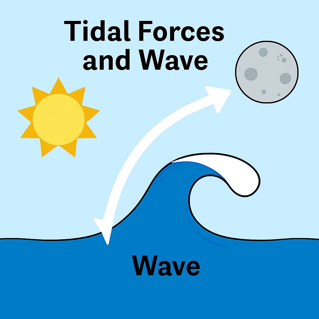
Fig. 29 **Figure 5.7 **: Tidal wave Analysis.#
Tidal Harmonic Analysis and Model Fitting#
Overview#
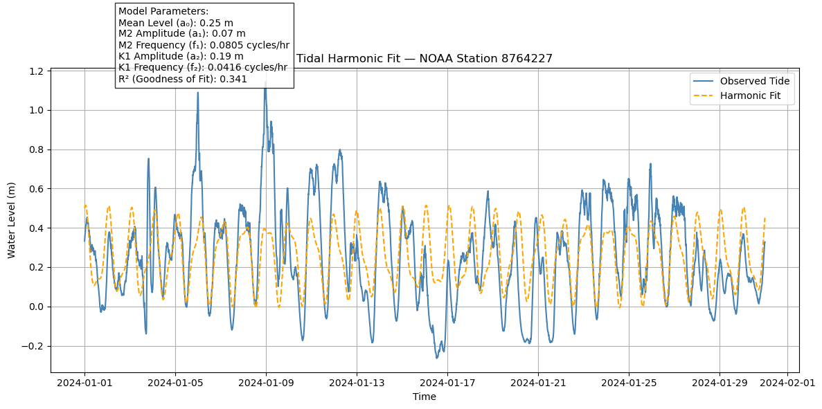
This analysis uses observed water level data from the NOAA Tides & Currents API to fit a harmonic tidal model. The model captures the dominant tidal constituents and estimates a smooth tidal signal. It also evaluates the goodness of fit using the coefficient of determination \(( R^2 \)).
Data Source#
Station: New Canal Station, New Orleans, LA (ID: 8764227)
Time Period: January 1–30, 2024
Datum: Mean Lower Low Water (MLLW)
Units: Metric
Interval: Hourly
Data is retrieved using NOAA’s official API and parsed into a pandas DataFrame.
Harmonic Tidal Model#
The model includes two primary tidal constituents:
M2: Principal lunar semidiurnal (period ≈ 12.42 hours)
K1: Lunar diurnal (period ≈ 23.93 hours)
🔹 Model Equation#
Where:
\(( a_0 \)): Mean water level
\(( a_1, a_2 \)): Amplitudes of M2 and K1 constituents
\(( f_1, f_2 \)): Frequencies (cycles per hour)
\(( p_1, p_2 \)): Phase shifts (radians)
\(( t \)): Time in hours since start of record
References#
[Pugh, 1987] offers a scientific foundation for tidal prediction using harmonic analysis, response methods, and tide-surge interactions, emphasizing theoretical rigor and observational techniques. [] USACE (2002) provides engineering-focused guidance, integrating tidal data into coastal design via numerical models like ADCIRC, with emphasis on practical applications and infrastructure planning.
2. Simulation#
🌊 NOAA Tidal Harmonic Analysis — Summary#
🧠 What It Is#
This script:
Fetches hourly water level data from NOAA’s New Canal Station in New Orleans
Fits a two-constituent harmonic model (M2 and K1 tides)
Visualizes observed vs. modeled tide data
Calculates goodness of fit (R²) to assess model accuracy
⚙️ How It Works#
Data Retrieval:
Uses NOAA API with station ID, time range, datum (
MLLW), and hourly intervalParses CSV response and extracts verified water levels
Time Conversion:
Converts timestamps to hours since initial record
Harmonic Fit:
Models tide as the sum of:
M2 (semi-diurnal)
K1 (diurnal)
Uses
scipy.curve_fitto optimize parameters
Fit Evaluation:
Computes R² to indicate match quality
Adds overlay of predicted tide line in plot
📊 Inputs#
Variable |
Value |
|---|---|
|
8764227 (New Canal, New Orleans) |
|
2024-01-01 |
|
2024-01-30 |
|
MLLW |
|
Hourly |
📈 Outputs#
Plot showing:
Blue curve: observed tide
Orange dashed: harmonic fit
Annotated parameters:
Mean level (a₀)
M2 and K1 amplitudes and frequencies
R² value — indicates how well the harmonic model explains observed variations
🧭 Interpretation#
High R² (near 1) → harmonic model fits observed tides well
Differences suggest:
Weather-driven anomalies
Additional tidal constituents
Local hydrodynamic complexity
This workflow is useful for validating tidal predictions, calibrating local models, or teaching harmonic tide principles.
import requests
import pandas as pd
import numpy as np
import matplotlib.pyplot as plt
from scipy.optimize import curve_fit
from io import StringIO

# 📍 NOAA Station Info
station_id = "8764227"        # New Canal Station, New Orleans LA
start_date = "20240101"
end_date   = "20240130"
datum      = "MLLW"
units      = "Metric"
interval   = "h"
timezone   = "GMT"

# 🌐 NOAA Data Browser Link
data_link = (
    f"https://tidesandcurrents.noaa.gov/waterlevels.html?"
    f"id={station_id}&units={units}&bdate={start_date}"
    f"&edate={end_date}&timezone={timezone}&datum={datum}&interval={interval}&action="
)
print("🔗 NOAA Water Level Data Link:")
print(data_link)

# 🛰️ NOAA API Setup
api_url = "https://api.tidesandcurrents.noaa.gov/api/prod/datagetter"
params = {
    "station": station_id,
    "begin_date": start_date,
    "end_date": end_date,
    "datum": datum,
    "product": "water_level",
    "application": "CopilotTideFit",
    "time_zone": timezone,
    "units": units,
    "format": "csv",
    "interval": interval
}

# 📡 Request Data
response = requests.get(api_url, params=params)

# 🧪 Check for API errors
if "error" in response.text.lower() or "Error" in response.text:
    print("❌ NOAA API returned an error:")
    print(response.text)
    raise ValueError("NOAA API error — check station ID, date range, or parameters.")

# 🧾 Load CSV into DataFrame
df = pd.read_csv(StringIO(response.text))

# 🔍 Identify Water Level Column
possible_cols = [c for c in df.columns if "Water Level" in c or "Observed" in c or "Verified" in c]
level_col = possible_cols[0] if possible_cols else None

if not level_col:
    print("❌ Could not find a valid water level column.")
    print(df.head())
    raise KeyError("Water level column not found in NOAA response.")

# 🕒 Time conversion
df["datetime"] = pd.to_datetime(df["Date Time"])
df["hours"] = (df["datetime"] - df["datetime"].iloc[0]).dt.total_seconds() / 3600
df["level"] = df[level_col]
df = df.dropna(subset=["level"])

# 🎯 Harmonic Model: Two tidal constituents (M2 + K1)
def harmonic_model(t, a0, a1, f1, p1, a2, f2, p2):
    return a0 + a1 * np.sin(2 * np.pi * f1 * t + p1) + a2 * np.sin(2 * np.pi * f2 * t + p2)

# 🔧 Fit model
initial_guess = [0, 0.5, 1/12.42, 0, 0.2, 1/23.93, 0]
params, _ = curve_fit(harmonic_model, df["hours"], df["level"], p0=initial_guess)
df["tidal_fit"] = harmonic_model(df["hours"], *params)

# 📈 Goodness of fit (R²)
residuals = df["level"] - df["tidal_fit"]
ss_res = np.sum(residuals**2)
ss_tot = np.sum((df["level"] - np.mean(df["level"]))**2)
r_squared = 1 - (ss_res / ss_tot)

# 📊 Plotting
plt.figure(figsize=(12, 6))
plt.plot(df["datetime"], df["level"], label="Observed Tide", color="steelblue")
plt.plot(df["datetime"], df["tidal_fit"], label="Harmonic Fit", linestyle="--", color="orange")
plt.xlabel("Time")
plt.ylabel("Water Level (m)")
plt.title(f"Tidal Harmonic Fit — NOAA Station {station_id}")

# 📌 Annotate model parameters
a0, a1, f1, p1, a2, f2, p2 = params
param_text = (
    f"Model Parameters:\n"
    f"Mean Level (a₀): {a0:.2f} m\n"
    f"M2 Amplitude (a₁): {a1:.2f} m\n"
    f"M2 Frequency (f₁): {f1:.4f} cycles/hr\n"
    f"K1 Amplitude (a₂): {a2:.2f} m\n"
    f"K1 Frequency (f₂): {f2:.4f} cycles/hr\n"
    f"R² (Goodness of Fit): {r_squared:.3f}"
)
plt.text(df["datetime"].iloc[int(len(df)/20)], max(df["level"]), param_text,
         fontsize=10, bbox=dict(facecolor='white', alpha=0.8))

plt.legend()
plt.grid(True)
plt.tight_layout()
plt.show()
🔗 NOAA Water Level Data Link:
https://tidesandcurrents.noaa.gov/waterlevels.html?id=8764227&units=Metric&bdate=20240101&edate=20240130&timezone=GMT&datum=MLLW&interval=h&action=
3. Simulation#
🌊 NOAA Tidal Amplitude Map Viewer — Coastal Station Explorer#
🧠 What It Is#
This Jupyter-based tool creates an interactive geospatial map of tidal constituent amplitudes (M2 and K1) for selected NOAA stations across the U.S. coastline.
⚙️ How It Works#
Defines station metadata: ID, name, latitude, longitude, and amplitudes of two tidal constituents:
M2_amp: semidiurnal tide amplitudeK1_amp: diurnal tide amplitude
Uses Cartopy for geographic plotting
Provides a dropdown widget to choose the tidal constituent for display
Plots stations as colored markers, scaled by amplitude values
🎛️ Inputs#
Input |
Description |
|---|---|
|
Choose either |
📊 Outputs#
📍 Map showing station locations across U.S. coastline
🌈 Color scale representing selected tidal amplitude (in meters)
📌 Station names labeled next to markers
🧭 Coastline, state borders, and map extent from West to East Coast
🧭 How to Interpret#
Darker markers → higher tidal amplitude
Useful for:
Understanding regional variation in tidal energy
Comparing semidiurnal vs diurnal dominance
Site selection for tidal studies or coastal modeling
This visualization links geographic context to tidal dynamics—making station-level tidal variation intuitively accessible.
import pandas as pd
import matplotlib.pyplot as plt
import cartopy.crs as ccrs
import cartopy.feature as cfeature
import ipywidgets as widgets
from IPython.display import display, clear_output

# 📊 Sample NOAA station data
data = {
    "Station ID": ["8764227", "8771450", "9414290", "8410140", "8443970"],
    "Name": ["New Orleans", "Galveston", "San Francisco", "The Battery, NY", "Boston, MA"],
    "Latitude": [30.03, 29.3, 37.8, 40.7, 42.36],
    "Longitude": [-90.1, -94.8, -122.4, -74.0, -71.05],
    "M2_amp": [0.24, 0.31, 0.65, 1.4, 1.2],  # M2 amplitude in meters
    "K1_amp": [0.08, 0.12, 0.22, 0.3, 0.25]   # K1 amplitude in meters
}
stations = pd.DataFrame(data)

# 🎛️ Interactive plotting function
def plot_tidal_map(constituent):
    clear_output(wait=True)

    fig = plt.figure(figsize=(12, 8))
    ax = plt.axes(projection=ccrs.PlateCarree())
    ax.set_extent([-130, -65, 20, 52], crs=ccrs.PlateCarree())
    ax.add_feature(cfeature.COASTLINE)
    ax.add_feature(cfeature.BORDERS, linestyle=":")
    ax.add_feature(cfeature.STATES, edgecolor="gray")

    # 🎯 Plot stations colored by selected amplitude
    sc = ax.scatter(
        stations["Longitude"], stations["Latitude"],
        c=stations[constituent], s=100, edgecolor="k", cmap="viridis",
        label=f"{constituent} Amplitude"
    )

    for i, row in stations.iterrows():
        ax.text(row["Longitude"] + 0.5, row["Latitude"], row["Name"], fontsize=9)

    plt.colorbar(sc, label=f"{constituent.replace('_amp', '')} Amplitude (m)", shrink=0.6)
    plt.title(f"U.S. Coastal Stations — {constituent.replace('_amp', '')} Tidal Constituent Amplitude")
    plt.grid(True)
    plt.tight_layout()
    plt.show()

# 🎚️ Dropdown for constituent selection
constituent_dropdown = widgets.Dropdown(
    options={"M2 (semidiurnal)": "M2_amp", "K1 (diurnal)": "K1_amp"},
    value="M2_amp",
    description="Constituent:"
)

# 🔄 Display interactive map
interactive_map = widgets.interactive(plot_tidal_map, constituent=constituent_dropdown)
display(interactive_map)
4. Simulation#
Tidal Harmonic Model Description (Interactive Simulator)#
This enhanced tidal model demonstrates how key astronomical constituents contribute to tidal variation over time at coastal locations.
Overview#
The model simulates tidal elevation using four dominant harmonic components:
M2: Lunar semidiurnal (≈12.42 hours)
S2: Solar semidiurnal (12 hours)
K1: Lunar-solar diurnal (≈23.93 hours)
O1: Lunar declinational diurnal (≈25.82 hours)
These constituents represent the most influential cycles in global tide patterns. Combining them creates a realistic synthetic tide signal.
Interactive Features#
Built with ipywidgets, this simulator allows users to:
Dynamically adjust each constituent’s amplitude
Instantly see changes in the 7-day tidal curve
Explore how tidal patterns evolve with changing forces
Sliders for:
M2_amp: Semidiurnal lunar force (default = 0.4 m)S2_amp: Semidiurnal solar force (default = 0.2 m)K1_amp: Diurnal lunar-solar force (default = 0.2 m)O1_amp: Diurnal lunar declination (default = 0.1 m)
Mathematical Model#
The tidal height \(( H(t) \)) at time ( t ) (in hours) is given by:
Where:
\(( a_0 \)): Mean sea level (set to 0 in simulation)
\(( a_1, a_2, a_3, a_4 \)): Amplitudes for M2, S2, K1, O1 respectively
\(( f_1, f_2, f_3, f_4 \)): Frequencies (cycles per hour) for each constituent
Visualization#
The plot shows:
Tidal elevation over a simulated 7-day period
How interacting cycles create realistic peaks, troughs, and asymmetry
Effects of adjusting lunar vs. solar forces in real time
The x-axis represents time, and the y-axis shows synthetic water level in meters.
Why Use This Model?#
This tool is ideal for:
Educators teaching tidal dynamics
Coastal engineers exploring wave-tide interaction
Students studying harmonic analysis of ocean systems
Anyone curious about how the Moon and Sun shape Earth’s tides
It provides an intuitive interface and mathematically grounded framework for exploring tides without requiring raw observational data.
import numpy as np
import matplotlib.pyplot as plt
from datetime import datetime, timedelta
from ipywidgets import FloatSlider, interact
import matplotlib.dates as mdates

# Time setup: simulate 7 days with hourly resolution
hours = np.arange(0, 7 * 24 + 1)
start = datetime(2024, 1, 1)
time_stamps = [start + timedelta(hours=int(h)) for h in hours]

# Tidal constituent frequencies (cycles per hour)
frequencies = {
    'M2': 1 / 12.42,
    'S2': 1 / 12.00,
    'K1': 1 / 23.93,
    'O1': 1 / 25.82
}

# Tidal model with multiple constituents
def multi_tide_model(hours, M2_amp, S2_amp, K1_amp, O1_amp):
    tide = (
        M2_amp * np.sin(2 * np.pi * frequencies['M2'] * hours) +
        S2_amp * np.sin(2 * np.pi * frequencies['S2'] * hours) +
        K1_amp * np.sin(2 * np.pi * frequencies['K1'] * hours) +
        O1_amp * np.sin(2 * np.pi * frequencies['O1'] * hours)
    )
    return tide

# Plotting function
def plot_tide(M2_amp, S2_amp, K1_amp, O1_amp):
    tide = multi_tide_model(hours, M2_amp, S2_amp, K1_amp, O1_amp)
    fig, ax = plt.subplots(figsize=(12, 4))
    ax.plot(time_stamps, tide, color='royalblue')
    ax.set_title("Enhanced Tidal Model — M2, S2, K1, O1")
    ax.set_xlabel("Time")
    ax.set_ylabel("Water Level (m)")
    ax.xaxis.set_major_formatter(mdates.DateFormatter('%b %d'))
    ax.grid(True)
    plt.tight_layout()
    plt.show()

# Interactive sliders
interact(plot_tide,
         M2_amp=FloatSlider(value=0.4, min=0.0, max=1.0, step=0.01, description='M2 Amp'),
         S2_amp=FloatSlider(value=0.2, min=0.0, max=1.0, step=0.01, description='S2 Amp'),
         K1_amp=FloatSlider(value=0.2, min=0.0, max=1.0, step=0.01, description='K1 Amp'),
         O1_amp=FloatSlider(value=0.1, min=0.0, max=1.0, step=0.01, description='O1 Amp'));
5. Self-Assessment#
Quiz: Tidal Harmonic Analysis and Model Fitting#
Test your understanding of harmonic tidal modeling using NOAA coastal data.
Conceptual Questions#
What is the primary purpose of the harmonic tidal model described in the analysis?
A. To predict weather patterns
✅ B. To capture dominant tidal constituents and estimate a smooth tidal signal
C. To measure ocean salinity levels
D. To analyze wave heights during storms
Which tidal constituent has a period of approximately 12.42 hours?
A. K1
✅ B. M2
C. S2
D. O1
What does the coefficient of determination ( R^2 ) indicate in the context of the tidal model?
A. The accuracy of the API data retrieval
✅ B. The strength of the fit between observed and modeled tidal levels
C. The frequency of tidal constituents
D. The amplitude of tidal waves
What is the role of ( a_0 ) in the harmonic tidal model equation?
A. It represents the amplitude of the tidal constituents
✅ B. It represents the mean water level
C. It represents the frequency of the tidal constituents
D. It represents the phase shift of the tidal constituents
Which method is used to fit the harmonic tidal model to the observed data?
A. Linear regression
✅ B. Nonlinear least squares
C. Fourier transform
D. Wavelet analysis
What does the term ( f_1 ) represent in the harmonic tidal model equation?
A. The amplitude of the tidal constituent
✅ B. The frequency of the tidal constituent
C. The phase shift of the tidal constituent
D. The mean water level
Why are M2 and K1 chosen as the primary tidal constituents in the model?
A. They are the only tidal constituents available in NOAA data
✅ B. They represent the most significant semidiurnal and diurnal tidal components
C. They have the longest periods among all tidal constituents
D. They are easier to model than other tidal constituents
What is the significance of the phase shift ( p_1 ) in the harmonic tidal model?
A. It determines the amplitude of the tidal constituent
✅ B. It adjusts the timing of the tidal constituent’s peak
C. It represents the frequency of the tidal constituent
D. It sets the baseline water level
What does the term ( t ) represent in the harmonic tidal model equation?
A. The amplitude of the tidal constituent
✅ B. The time in hours since the start of the record
C. The frequency of the tidal constituent
D. The phase shift of the tidal constituent
What is the primary advantage of using a harmonic tidal model?
A. It eliminates the need for observed data
✅ B. It provides a smooth and predictive representation of tidal behavior
C. It measures ocean salinity levels
D. It predicts weather patterns
🌊 Tidal Harmonic Model Description (Interactive Simulator)#
This enhanced tidal model demonstrates how key astronomical constituents contribute to tidal variation over time at coastal locations.
📘 Overview#
The model simulates tidal elevation using four dominant harmonic components:
M2: Lunar semidiurnal (≈12.42 hours)
S2: Solar semidiurnal (12 hours)
K1: Lunar-solar diurnal (≈23.93 hours)
O1: Lunar declinational diurnal (≈25.82 hours)
These constituents represent the most influential cycles in global tide patterns. Combining them creates a realistic synthetic tide signal.
🎛️ Interactive Features#
Built with ipywidgets, this simulator allows users to:
Dynamically adjust each constituent’s amplitude
Instantly see changes in the 7-day tidal curve
Explore how tidal patterns evolve with changing forces
Sliders for:
M2_amp: Semidiurnal lunar force (default = 0.4 m)S2_amp: Semidiurnal solar force (default = 0.2 m)K1_amp: Diurnal lunar-solar force (default = 0.2 m)O1_amp: Diurnal lunar declination (default = 0.1 m)
📐 Mathematical Model#
The tidal height \(( H(t) \)) at time ( t ) (in hours) is given by:
Where:
\(( a_0 \)): Mean sea level (set to 0 in simulation)
\(( a_1, a_2, a_3, a_4 \)): Amplitudes for M2, S2, K1, O1 respectively
\(( f_1, f_2, f_3, f_4 \)): Frequencies (cycles per hour) for each constituent
📈 Visualization#
The plot shows:
Tidal elevation over a simulated 7-day period
How interacting cycles create realistic peaks, troughs, and asymmetry
Effects of adjusting lunar vs. solar forces in real time
The x-axis represents time, and the y-axis shows synthetic water level in meters.
🧪 Why Use This Model?#
This tool is ideal for:
Educators teaching tidal dynamics
Coastal engineers exploring wave-tide interaction
Students studying harmonic analysis of ocean systems
Anyone curious about how the Moon and Sun shape Earth’s tides
It provides an intuitive interface and mathematically grounded framework for exploring tides without requiring raw observational data.
import numpy as np
import matplotlib.pyplot as plt
from datetime import datetime, timedelta
from ipywidgets import FloatSlider, interact
import matplotlib.dates as mdates

# Time setup: simulate 7 days with hourly resolution
hours = np.arange(0, 7 * 24 + 1)
start = datetime(2024, 1, 1)
time_stamps = [start + timedelta(hours=int(h)) for h in hours]

# Tidal constituent frequencies (cycles per hour)
frequencies = {
    'M2': 1 / 12.42,
    'S2': 1 / 12.00,
    'K1': 1 / 23.93,
    'O1': 1 / 25.82
}

# Tidal model with multiple constituents
def multi_tide_model(hours, M2_amp, S2_amp, K1_amp, O1_amp):
    tide = (
        M2_amp * np.sin(2 * np.pi * frequencies['M2'] * hours) +
        S2_amp * np.sin(2 * np.pi * frequencies['S2'] * hours) +
        K1_amp * np.sin(2 * np.pi * frequencies['K1'] * hours) +
        O1_amp * np.sin(2 * np.pi * frequencies['O1'] * hours)
    )
    return tide

# Plotting function
def plot_tide(M2_amp, S2_amp, K1_amp, O1_amp):
    tide = multi_tide_model(hours, M2_amp, S2_amp, K1_amp, O1_amp)
    fig, ax = plt.subplots(figsize=(12, 4))
    ax.plot(time_stamps, tide, color='royalblue')
    ax.set_title("Enhanced Tidal Model — M2, S2, K1, O1")
    ax.set_xlabel("Time")
    ax.set_ylabel("Water Level (m)")
    ax.xaxis.set_major_formatter(mdates.DateFormatter('%b %d'))
    ax.grid(True)
    plt.tight_layout()
    plt.show()

# Interactive sliders
interact(plot_tide,
         M2_amp=FloatSlider(value=0.4, min=0.0, max=1.0, step=0.01, description='M2 Amp'),
         S2_amp=FloatSlider(value=0.2, min=0.0, max=1.0, step=0.01, description='S2 Amp'),
         K1_amp=FloatSlider(value=0.2, min=0.0, max=1.0, step=0.01, description='K1 Amp'),
         O1_amp=FloatSlider(value=0.1, min=0.0, max=1.0, step=0.01, description='O1 Amp'));