
Chapter 5 Coastal Engineering: Wave Kinematics#
1. Introduction#
🌊 Wave Kinematics#
Several wave theories are used to characterize the profile, kinematics, energy, and other dynamic parameters of water waves. These theories are typically categorized based on the linearity of the wave motion.
Airy (Linear) Theory - Assumes wave symmetry about the still water level. - Described using a cosine function. - Models only oscillatory waves. - Applicable to deep water and low-amplitude conditions. - Simple and widely used in engineering design. - May oversimplify results due to idealized assumptions.
📘 About Linear Wave Theory#
Linear Wave Theory (Airy wave theory) describes the propagation of small-amplitude waves on the surface of an inviscid, incompressible, and irrotational fluid. It assumes:
Small Amplitude Waves: \(( H \ll \lambda \)), \(( H \ll h \))
Incompressible Fluid: Constant density
Irrotational Flow: No internal vorticity
Homogeneous Properties: Uniform throughout
Gravity Waves: Dominated by gravitational restoring forces
Assumes small-amplitude, symmetric, oscillatory waves about the still water level, typically modeled with cosine functions. It is simple, analytically tractable, and widely used in engineering design—especially for deep water and low-steepness waves. However, it oversimplifies some physical phenomena due to its assumptions
🔬 Governing Equations#
Laplace’s Equation for velocity potential \(( \phi \)):
$\( \nabla^2 \phi = 0 \)$Free Surface Boundary Condition:
$\( \frac{\partial \phi}{\partial t} + g\eta = 0 \quad \text{at } z = \eta \)$Bottom Boundary Condition:
$\( \frac{\partial \phi}{\partial z} = 0 \quad \text{at } z = -h \)$
📈 Wave Solutions#
Surface Elevation:
$\( \eta(x, t) = a \cos(kx - \omega t) \)$Velocity Potential:
$\( \phi(x, z, t) = \frac{a g}{\omega} \cosh(k(z + h)) \cos(kx - \omega t) \)$Dispersion Relation:
$\( \omega^2 = gk \tanh(kh) \)$
Where:
\(( a \)): Wave amplitude
\(( k = \dfrac{2\pi}{\lambda} \)): Wave number
\(( \omega = 2\pi f \)): Angular frequency
\(( h \)): Water depth
\(( g \)): Acceleration due to gravity
📚 Reference#
[U.S. Army Corps of Engineers, 1984] introduces Airy (linear) wave theory and applies it to coastal design, forming the basis for wave force calculations on structures. [Dean and Dalrymple, 2001] offers a rigorous description of wave kinematics, especially through the lens of Airy (linear) wave theory. It derives analytical expressions for surface elevation, velocity, acceleration, and pressure beneath waves, assuming small amplitude and inviscid, irrotational flow. The book clearly explains the physical meaning of each term and boundary condition, making it ideal for engineering applications. It also connects linear theory to more advanced models, providing a solid foundation for understanding wave-structure interactions and coastal processes.
2. Simulation#
🌊 Interactive Wave Field Simulator — Airy Theory Visualization#
A dynamic Jupyter Notebook tool that simulates and visualizes wave-induced kinematics and pressure fields in a 2D domain using Airy wave theory.
⚙️ How It Works#
Defines spatial grid in horizontal (x) and vertical (z) directions
Computes:
Surface elevation ζ
Horizontal velocity (u)
Horizontal acceleration (aₓ)
Hydrostatic + dynamic pressure (p)
Uses sinusoidal expressions for wave motion and hyperbolic functions for vertical decay
Visualizes outputs as:
Line plot of surface elevation
Heatmaps for velocity, acceleration, and pressure distributions
🎛️ Inputs (via Sliders)#
Input |
Meaning |
|---|---|
|
Phase time of wave cycle |
|
Surface wave amplitude |
|
Water depth |
📊 Outputs#
ζ(x): Surface elevation vs. horizontal distance
u(x, z): Velocity field heatmap
aₓ(x, z): Acceleration field heatmap
p(x, z): Pressure field heatmap
🧭 Interpretation#
Velocity and pressure decay with depth due to hyperbolic attenuation
Surface elevation shows sinusoidal wave form at selected time
Use outputs to:
Visualize wave structure and impact at different depths
Explore nearshore hydrodynamics
Validate linear theory assumptions
Ideal for education, coastal planning, and understanding wave-driven forces beneath the surface.
import numpy as np
import plotly.graph_objects as go
import plotly.express as px
from ipywidgets import interact, FloatSlider
import ipywidgets as widgets
from IPython.display import display
import plotly.graph_objects as go
# Define all constant/parameters; grid size
nz = 100 # number of grid along z-axis
nx = 100 # number of grid along x-axis
g = 9.81
freq=1     # Hz frequency
omega = 2 * np.pi * freq
k = omega**2 / g
zetaA=0.2  # wave amplitude
ts=0       # time start
te=4*np.pi # terminal time
d=2       # water depth
xe=5     # maximum range
time=2.   # ref time
x=0
k=omega**2/g

############ Grid####################
x = np.linspace(0, xe, nx)
z = np.linspace(-d, 0, nz)

# Compute spatial distribution of velocity, accleration and pressure
def compute_fields(time,zetaA,d):
    rho = 1000# density of water in kg/m^3
    zeta=zetaA*np.sin(omega*time-k*x)
    u=np.zeros((nx,nz))
    ax=np.zeros((nx,nz))
    p=np.zeros((nx,nz))
    sp=np.zeros((nx,nz))
    H = 2 * zetaA
    #print(nx,nz,k,d,time,zetaA,omega)
    for iz in range(nz):
        for ix in range(nx):
            u[ix, iz]=zetaA*omega*np.cosh(k*(z[iz]+d))/np.cosh(k*d)*np.cos(omega*time-k*x[ix])
            #p[ix,iz] = rho * g * (-z[iz]) + 0.5 * rho * u[ix, iz]**2
            p[ix, iz] = -rho * g * z[iz] + rho * g * H / np.cosh(k * d) * np.cosh(k * (d + z[iz])) * np.cos(k * x[ix] - omega * time)
            #sp[ix,iz] = omega/k*np.sqrt(np.cosh(k*d)/np.cosh(k*(z[ix]+d)))
            ax[ix, iz]=zetaA*omega**2*np.cosh(k*(z[iz]+d))/np.cosh(k*d)*np.cos(omega*time-k*x[ix])
    return zeta, u, ax, p,sp

# Interactive plotting function
def plot_interactive(time, zetaA, d):
    global z
    z = np.linspace(-d, 0, nz)# update z based on depth
    zeta, u, ax,p,sp = compute_fields(time, zetaA, d)
    fig = go.Figure()
    # Surface elevation plot
    fig.add_trace(go.Scatter(x=x, y=zeta, mode='lines', name='water surface ζ',
                             line=dict(color='blue')))
    fig.update_layout(title='Water Surface ζ [m]',
                      xaxis_title='distance [m]',
                      yaxis_title='Surface ζ [m]',
                      height=300)

    fig.show()
    # Velocity field plot
    fig_u = px.imshow(u.T, origin='lower', aspect='auto', color_continuous_scale='Jet',labels={'color': 'u [m/s]'})
    fig_u.update_layout(title='Velocity Field u [m/s]', xaxis_title='x [m]', yaxis_title='z [m]')
    fig_u.update_xaxes(tickvals=np.linspace(0, nx-1, 5),ticktext=[f"{val:.1f}" for val in np.linspace(0, xe, 5)])
    fig_u.update_yaxes(tickvals=np.linspace(0, nz-1, 5),ticktext=[f"{val:.1f}" for val in np.linspace(-d, 0, 5)])
    fig_u.show()
    # Acceleration field plot
    fig_ax = px.imshow(ax.T, origin='lower', aspect='auto', color_continuous_scale='Jet',labels={'color': 'w [m/s²]'})
    fig_ax.update_layout(title='Acceleration Field w [m/s²]',xaxis_title='x [m]',yaxis_title='z [m]')
    fig_ax.update_xaxes(tickvals=np.linspace(0, nx-1, 5),ticktext=[f"{val:.1f}" for val in np.linspace(0, xe, 5)])
    fig_ax.update_yaxes(tickvals=np.linspace(0, nz-1, 5), ticktext=[f"{val:.1f}" for val in np.linspace(-d, 0, 5)])
    fig_ax.show()
    # pressure field plot

    fig = go.Figure(data=go.Heatmap(z=p.T,colorscale='Jet',colorbar=dict(title='p [pascal]')))
    fig.update_layout( title='Pressure Field Pascal [Pa]',xaxis_title='x [m]',yaxis_title='z [m]',height=400)
    fig.update_xaxes(tickvals=np.linspace(0, nx-1, 5),ticktext=[f"{val:.1f}" for val in np.linspace(0, xe, 5)])
    fig.update_yaxes(tickvals=np.linspace(0, nz-1, 5),ticktext=[f"{val:.1f}" for val in np.linspace(-d, 0, 5)])
    fig.show()

# Create interactive slider with all parameters
time_slider = widgets.FloatSlider(value=2.0, min=0, max=4*np.pi, step=0.1, description='Time [s]')
zeta_slider = widgets.FloatSlider(value=0.2, min=0.1, max=4, step=0.1, description='Amplitude [m]')
depth_slider = widgets.FloatSlider(value=2.0, min=1, max=10, step=0.1, description='Depth [m]')
run_button = widgets.Button(description="Run Simulation")

# Output area
output = widgets.Output()

# Callback function
def on_button_click(b):
    with output:
        output.clear_output()
        plot_interactive(time_slider.value, zeta_slider.value, depth_slider.value)
run_button.on_click(on_button_click)
# Display widgets
display(widgets.VBox([time_slider, zeta_slider, depth_slider, run_button, output]))
import numpy as np
import matplotlib.pyplot as plt
from ipywidgets import interact, FloatSlider

# Constants
g = 9.81  # gravitational acceleration (m/s²)
rho = 1025  # seawater density (kg/m³)

def wave_properties(H, T, h, z):
    """
    Computes wave energy, power, and pressure at depth z using linear wave theory.
    """
    # Derived quantities
    omega = 2 * np.pi / T
    L = (g * T**2) / (2 * np.pi) * np.tanh((2 * np.pi * h) / (g * T**2))  # approximate dispersion
    k = 2 * np.pi / L
    c = L / T

    # Energy per unit area
    E_pot = (1/8) * rho * g * H**2
    E_kin = E_pot  # For linear theory, kinetic ≈ potential
    E_total = E_pot + E_kin

    # Wave power per unit crest length
    P = E_total * c

    # Pressure at depth z (z measured from still water level, negative downward)
    pressure = rho * g * H / 2 * np.cosh(k * (h + z)) / np.cosh(k * h)

    return L, c, E_pot, E_kin, E_total, P, pressure

def plot_wave_energy(H=2.0, T=8.0, h=10.0, z=-2.0):
    L, c, E_pot, E_kin, E_total, P, pressure = wave_properties(H, T, h, z)

    print(f"🌊 Wave Characteristics:")
    print(f"- Wavelength (L): {L:.2f} m")
    print(f"- Phase Speed (c): {c:.2f} m/s")
    print(f"\n⚡ Energy:")
    print(f"- Potential Energy: {E_pot:.2f} J/m²")
    print(f"- Kinetic Energy: {E_kin:.2f} J/m²")
    print(f"- Total Energy: {E_total:.2f} J/m²")
    print(f"- Wave Power: {P:.2f} W/m")
    print(f"\n🧭 Pressure at z = {z} m:")
    print(f"- Dynamic Pressure: {pressure:.2f} Pa")

    # Optional plot: pressure profile
    z_vals = np.linspace(-h, 0, 500)
    pressure_profile = rho * g * H / 2 * np.cosh(2 * np.pi / L * (h + z_vals)) / np.cosh(2 * np.pi / L * h)

    plt.figure(figsize=(6, 4))
    plt.plot(pressure_profile, z_vals)
    plt.title('Pressure Profile Under Wave (Linear Theory)')
    plt.xlabel('Pressure (Pa)')
    plt.ylabel('Depth z (m)')
    plt.grid(True)
    plt.gca().invert_yaxis()
    plt.tight_layout()
    plt.show()

interact(plot_wave_energy,
         H=FloatSlider(value=2.0, min=0.1, max=5.0, step=0.1, description='Wave Height H (m)'),
         T=FloatSlider(value=8.0, min=2.0, max=20.0, step=0.5, description='Wave Period T (s)'),
         h=FloatSlider(value=10.0, min=1.0, max=50.0, step=1.0, description='Water Depth h (m)'),
         z=FloatSlider(value=-2.0, min=-50.0, max=0.0, step=0.5, description='Depth z (m)'))
<function __main__.plot_wave_energy(H=2.0, T=8.0, h=10.0, z=-2.0)>
3. Self-Assessment#
Wave kinematics Conceptual Understanding#
Why does linear wave theory assume small-amplitude waves? What physical phenomena would invalidate this assumption?
What role does the velocity potential \(( \phi \)) play in describing wave motion?
How does the dispersion relation \(( \omega^2 = gk \tanh(kh) \)) help us distinguish between shallow and deep water waves?
Why does pressure beneath a wave include both hydrostatic and dynamic components?
How would increasing depth \(( h \)) affect the vertical structure of the velocity and acceleration fields?
What surprised you most when visualizing the pressure or velocity field?
Was it how deep the wave motion extended? Or how quickly the pressure varied with depth?When adjusting wave amplitude or depth, how did your intuition compare to what the simulation revealed?
Did you expect deeper motion at higher amplitudes, or more flattening at greater depths?How would you explain to a non-engineering friend why water particles in waves don’t move horizontally across the ocean?
How might real-world effects (e.g., wind, viscosity, turbulence) deviate from what you saw in the simulation?
Wave kinematics Quiz#
Q1: Which assumption is not part of linear wave theory?
A. The fluid is homogeneous
B. The wave height is large compared to the depth
C. The flow is irrotational
D. The fluid is incompressible
🟢 Answer: B
Q2: In the wave equation \(( \eta(x,t) = a \cos(kx - \omega t) \)), what does \(( a \)) represent?
A. Wavelength
B. Water depth
C. Wave amplitude
D. Velocity potential
🟢 Answer: C
Q3: What does the term \(( \cosh(k(z + h)) \)) control in the solution for velocity potential?
A. Time oscillation
B. Horizontal periodicity
C. Decay with depth
D. Wave energy
🟢 Answer: C
Q1. What does increasing the value of the Amplitude slider (ζₐ) do to the computed velocity and pressure fields?
It reduces both fields
It increases the surface wave speed only
It increases the magnitude of velocity and pressure
It has no effect on any field 🟢 Correct Answer: C
Q2. When using the Time slider, what type of behavior is observed in the surface elevation plot?
Linear increase with time
Random noise fluctuation
Cyclical or oscillatory motion
Constant wave crest height 🟢 Correct Answer: C
Q3. What effect does increasing the Water Depth (d) have on the shape of the velocity and acceleration fields?
Motion penetrates deeper and becomes more uniform
Particle velocity becomes vertical only
Pressure increases but velocity vanishes
Fields become zero beyond surface level 🟢 Correct Answer: A
Q4. At which depth zone is horizontal particle acceleration generally highest?
At the bottom (z = −d)
At the surface (z = 0)
Uniform at all depths
At mid-depth 🟢 Correct Answer: B
Q5. True or False: Increasing the wave amplitude will linearly increase pressure everywhere in the fluid column. 🟢 Correct Answer: False 💡 Explanation: Pressure depends on both hydrostatic and dynamic components, and the latter varies nonlinearly with depth and time.
Short Answer & Discussion Prompts#
What do you observe about the pressure field as time progresses? How does this relate to the position of wave crests and troughs?
Explain why acceleration and velocity fields attenuate with depth even though the wave propagates along the surface.
If the wavelength were longer (i.e., smaller k), how do you think the shape of the pressure field would change
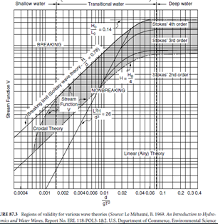
🌊 Wave Theory Applicability Quiz#
Instructions:#
For each question, use the given wave height (H) and water depth (h) to determine the most suitable wave theory. Choose from:
Linear (Airy) Theory
Stokes Theory
Cnoidal Theory
Solitary Wave Theory
Use the relative wave height \(( \frac{H}{h} \)) and relative depth \(( \frac{h}{L} \)) (where \(( L \)) is wavelength) to guide your choice.
❓ Question 1#
Given:
Wave height \(( H = 1.2 \, \text{m} \))
Water depth \(( h = 15 \, \text{m} \))
Wavelength \(( L = 100 \, \text{m} \))
Calculate:
\(( \frac{H}{h} = \_\_\_\_ \))
\(( \frac{h}{L} = \_\_\_\_ \))
Which wave theory is most applicable?
Linear (Airy) Theory
Stokes Theory
Cnoidal Theory
Solitary Wave Theory
❓ Question 2#
Given:
Wave height \(( H = 2.5 \, \text{m} \))
Water depth \(( h = 4 \, \text{m} \))
Wavelength \(( L = 40 \, \text{m} \))
Calculate:
\(( \frac{H}{h} = \_\_\_\_ \))
\(( \frac{h}{L} = \_\_\_\_ \))
Which wave theory is most applicable?
Linear (Airy) Theory
Stokes Theory
Cnoidal Theory
Solitary Wave Theory
❓ Question 3#
Given:
Wave height \(( H = 0.5 \, \text{m} \))
Water depth \(( h = 25 \, \text{m} \))
Wavelength \(( L = 150 \, \text{m} \))
Calculate:
\(( \frac{H}{h} = \_\_\_\_ \))
\(( \frac{h}{L} = \_\_\_\_ \))
Which wave theory is most applicable?
Linear (Airy) Theory
Stokes Theory
Cnoidal Theory
Solitary Wave Theory
✅ Answer Key (Optional)#
**Answers:**
1. Linear (Airy) Theory
2. Cnoidal Theory
3. Linear (Airy) Theory