
Chapter 3 Hydraulics: Seepage analysis#
1. Introduction#
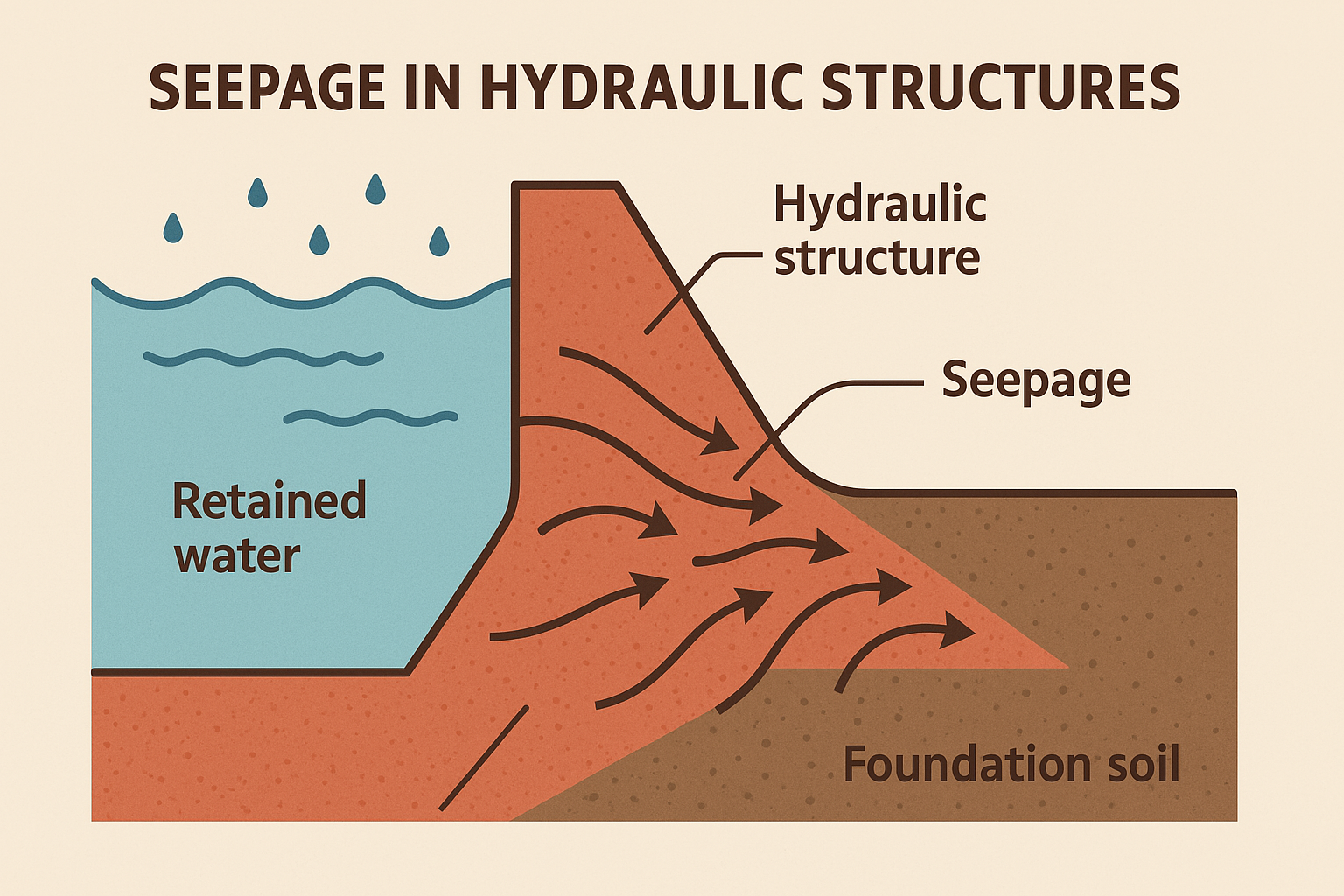
Fig. 8 ** Figure 3.4 **: Seepage Analysis.#
💧 Seepage in Hydraulic Structures#
Seepage refers to the slow movement of water through soil or porous media due to hydraulic gradients. It occurs naturally in embankments, foundations, and abutments of hydraulic structures such as dams, levees, and floodwalls.
⚠️ How Seepage Threatens Hydraulic Infrastructure#
Structure |
Seepage Risks |
|---|---|
Dams |
- Uplift pressure reduces stability |
Levees |
- Boiling and sand boils |
Floodwalls |
- Undermining of wall base |
🔍 Seepage Failure Mechanisms#
Piping: Progressive erosion of soil particles along seepage paths
Uplift: Vertical pressure that can lift slabs or destabilize foundations
Boiling: Upward flow causing soil to behave like a fluid
Saturation: Reduces shear strength and increases risk of slope failure
🧮 Methods for Seepage Analysis#
Method / Approach |
Description |
|---|---|
Flow Net Analysis |
Graphical method using equipotential and flow lines to estimate seepage quantity and pressure distribution |
Darcy’s Law |
Fundamental equation for flow through porous media: |
Finite Element Method (FEM) |
Numerical modeling of seepage through complex geometries and heterogeneous soils |
Finite Difference Method (FDM) |
Grid-based numerical solution of Laplace or Richards equations for steady/unsteady flow |
SEEP/W (GeoStudio) |
Commercial software for 2D/3D seepage modeling with boundary conditions and material properties |
Empirical Charts |
Used for estimating seepage through homogeneous embankments or foundations |
Critical Gradient Analysis |
Determines the gradient at which piping or boiling may initiate: |
🔍 Common Seepage Failure Mechanisms#
Mechanism |
Description |
|---|---|
Piping |
Soil particles eroded by seepage flow, forming internal channels |
Uplift Pressure |
Vertical pressure destabilizing slabs or foundations |
Boiling / Sand Boils |
Upward flow carrying soil to surface; precursor to piping |
Saturation |
Weakens soil shear strength; leads to slope failure |
Crack Propagation |
Seepage concentrates along cracks or conduits |
🧠 Lessons Learned#
Seepage failures often occur without overtopping
Many failures happen during first reservoir filling or within first 5 years
Monitoring and maintenance are critical to detect early signs
Relief wells, cutoff walls, and filters are essential for seepage control
Levee failures are often rapid and offer little warning time
🧠 Conceptual Insight#
Seepage is a hidden threat to hydraulic structures —
understanding its behavior is essential for designing safe embankments,
preventing failure, and ensuring long-term performance.
Reference#
[] provides a comprehensive resources for analyzing seepage beneath gravity dams. It outlines analytical methods such as Laplace’s equation and flow net construction to estimate seepage quantities, phreatic line locations, and exit gradients. The manual distinguishes between confined and unconfined flow scenarios, including cases of finite and infinite pervious foundations. It also details seepage control measures like cutoff trenches, grout curtains, drainage galleries, relief wells, and impervious blankets. This manual is a critical resource for civil engineers focused on dam design, safety evaluation, and geotechnical-hydraulic integration. [Novak et al., 2007] also moderately discussess the seepage under the structure and the methods.
2. Simulation#
💧 Interactive Dam Seepage Simulation — Laplace Equation#
This Python notebook cell simulates 2D steady-state seepage beneath a dam using the Laplace equation. It uses finite difference methods and ipywidgets to allow dynamic user control of geometry and boundary conditions.
🧠 Governing Equation#
We solve the Laplace equation:
Where:
\(( h \)): hydraulic head [m]
Assumptions:
Steady state
Homogeneous, isotropic medium
No flow across bottom and top boundaries
Constant head at upstream and downstream boundaries
⚙️ Inputs and Controls#
Parameter |
Description |
|---|---|
Grid Nx, Ny |
Number of grid points in x and y |
Domain Lx, Ly |
Length and depth of dam section (m) |
Head h_left |
Upstream boundary condition (m) |
Head h_right |
Downstream boundary condition (m) |
Users can adjust these interactively with sliders.
🔁 Solver Logic#
Discretize domain into a 2D grid.
Apply boundary conditions:
Upstream and downstream head fixed
Top and bottom boundaries are no-flow
Use Gauss-Seidel iteration until convergence.
📊 Visualization#
Hydraulic head is plotted using filled contours (
contourf).Vertical gradient beneath dam visualizes seepage potential.
Real-time interactivity enables design exploration.
🚀 Use Cases#
Estimate flow patterns beneath dams and levees
Demonstrate influence of geometry and boundary heads
Educational illustration of potential flow and Laplace solutions
import numpy as np
import matplotlib.pyplot as plt
import ipywidgets as widgets
from IPython.display import display

# 🔧 Finite difference solver with seepage face on downstream
def solve_laplace(Nx, Ny, h_left, h_right, tol=1e-4, max_iter=5000):
    h = np.zeros((Ny, Nx))

    # Initial boundary conditions
    h[:, 0] = h_left  # Upstream head
    h[:, -1] = np.linspace(h_right, h_right, Ny)  # Seepage face (free exit)

    for _ in range(max_iter):
        h_old = h.copy()

        # Update interior points
        for i in range(1, Ny - 1):
            for j in range(1, Nx - 1):
                h[i, j] = 0.25 * (h[i+1, j] + h[i-1, j] + h[i, j+1] + h[i, j-1])

        # Reapply boundary conditions
        h[:, 0] = h_left
        h[:, -1] = np.linspace(h_right, h_right, Ny)  # Seepage face
        h[0, :] = h[1, :]     # Bottom (no flow)
        h[-1, :] = h[-2, :]   # Top (no flow)

        if np.max(np.abs(h - h_old)) < tol:
            break

    return h

# 📊 Plot hydraulic head and streamline flow
def plot_seepage(Nx, Ny, Lx, Ly, h_left, h_right, K):
    if Nx < 2 or Ny < 2:
        print("⚠️ Grid size too small for seepage analysis.")
        return

    dx = Lx / (Nx - 1)
    dy = Ly / (Ny - 1)
    h = solve_laplace(Nx, Ny, h_left, h_right)
    X = np.linspace(0, Lx, Nx)
    Y = np.linspace(0, Ly, Ny)
    XX, YY = np.meshgrid(X, Y)

    # 💨 Darcy velocity field
    dh_dx, dh_dy = np.gradient(h, dx, dy)
    qx = -K * dh_dx
    qy = -K * dh_dy
    velocity_mag = np.sqrt(qx**2 + qy**2)

    # 🔢 Estimate seepage across downstream face
    seepage_rate = np.mean(qx[:, -1]) * Ly  # average flux × height

    # 📈 Plot head and streamlines
    plt.figure(figsize=(12, 5))
    contour = plt.contourf(XX, YY, h, levels=30, cmap="viridis")
    plt.colorbar(contour, label="Hydraulic Head (m)")
    plt.streamplot(XX, YY, qx, qy, color="white", density=1.2, linewidth=1)

    # 🔴 Velocity magnitude contours
    plt.contour(XX, YY, velocity_mag, levels=20, colors='red', linewidths=0.5)

    # 💬 Annotate seepage rate
    plt.text(Lx * 0.6, Ly * 0.1, f"Seepage Rate: {seepage_rate:.2f} m³/day",
             fontsize=12, color='white', bbox=dict(facecolor='black', alpha=0.5))

    plt.gca().invert_yaxis()
    plt.title("Seepage Flow & Streamlines with Seepage Face")
    plt.xlabel("Horizontal Distance (m)")
    plt.ylabel("Depth Beneath Dam (m)")
    plt.grid(True)
    plt.tight_layout()
    plt.show()

# 🎛️ Interactive controls
Nx_slider = widgets.IntSlider(value=100, min=50, max=200, step=10, description='Grid Nx')
Ny_slider = widgets.IntSlider(value=30, min=10, max=100, step=5, description='Grid Ny')
Lx_slider = widgets.FloatSlider(value=50.0, min=10.0, max=200.0, step=10.0, description='Length Lx (m)')
Ly_slider = widgets.FloatSlider(value=10.0, min=5.0, max=50.0, step=5.0, description='Depth Ly (m)')
h_left_slider = widgets.FloatSlider(value=10.0, min=1.0, max=20.0, step=0.5, description='Upstream Head (m)')
h_right_slider = widgets.FloatSlider(value=2.0, min=0.0, max=10.0, step=0.5, description='Downstream Head (m)')
K_slider = widgets.FloatSlider(value=1.0, min=0.01, max=10.0, step=0.1, description='Hydraulic Conductivity K')

ui = widgets.VBox([
    Nx_slider, Ny_slider, Lx_slider, Ly_slider,
    h_left_slider, h_right_slider, K_slider
])

out = widgets.interactive_output(plot_seepage, {
    'Nx': Nx_slider,
    'Ny': Ny_slider,
    'Lx': Lx_slider,
    'Ly': Ly_slider,
    'h_left': h_left_slider,
    'h_right': h_right_slider,
    'K': K_slider
})

display(ui, out)
3. Self-Assessment#
💧 Seepage Flow Analysis Beneath a Dam: Interpretation & Learning#
This module explores 2D seepage beneath a dam using a finite difference solution to Laplace’s equation, with a downstream seepage face. The model visualizes hydraulic head, streamlines, and velocity contours, and estimates total seepage rate.
📘 How to Interpret the Results#
🔹 Hydraulic Head Contours#
Represent the equipotential lines of groundwater flow.
Head decreases from upstream (left) to downstream (right).
Steep gradients indicate high flow velocity.
🔹 Streamlines#
Show the path of water particles through the soil.
Flow converges toward the downstream face, especially near the base.
Streamlines bend near boundaries due to no-flow conditions.
🔹 Velocity Magnitude Contours#
Red lines show zones of high seepage velocity.
Concentrated near the toe of the dam and seepage face.
Useful for identifying potential piping or erosion zones.
🔹 Seepage Rate#
Calculated as average horizontal Darcy flux across the downstream face: \( Q_{\text{seepage}} = \bar{q}_x \cdot L_y \)
Reported in m³/day — useful for drainage design and safety checks.
✅ Conceptual Questions#
What equation governs steady-state seepage in saturated soils?
A. Navier-Stokes
B. Laplace’s equation
C. Bernoulli’s equation
D. Richards’ equation
What boundary condition is applied at the bottom and top of the domain?
A. Constant head
B. No-flow (Neumann)
C. Seepage face
D. Free surface
Which parameter most directly affects the magnitude of seepage?
A. Grid resolution
B. Hydraulic conductivity
C. Upstream head
D. Depth of dam
Why is the downstream face modeled as a seepage face?
A. To simulate rainfall infiltration
B. To allow free exit of groundwater
C. To enforce zero velocity
D. To model impermeable boundary
🔍 Reflection Questions#
How does changing the upstream head affect the flow field and seepage rate?
Why is it important to visualize both head and velocity in seepage analysis?
What physical processes are captured by Laplace’s equation that uniform flow models ignore?
How would you modify this model to include anisotropic soils or layered media?
What are the risks of underestimating seepage beneath hydraulic structures?
💡 Engineering Insight#
“Seepage beneath dams is a critical safety concern. Visualizing flow paths and gradients helps engineers design effective drainage systems and prevent piping, uplift, and structural failure.”