
Chapter 2 Hydrology: Habitat Analysis#
1. Introduction#
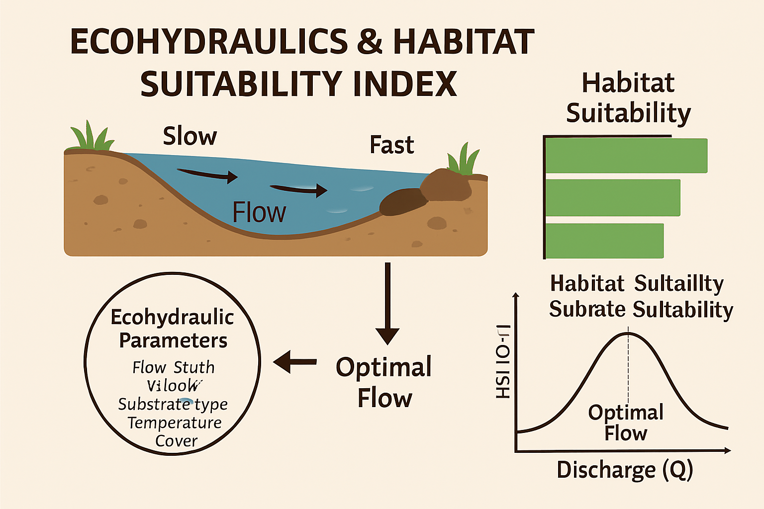
Fig. 5 ** Figure 2.5 **: Eco-Hydraulics and Habitat Suitability Index.#
🌿 Habitat Analysis and Hydraulics: Concepts and Methods#
Human interventions like dam construction, channelization, and river regulation aim to reduce natural flow variability for flood control, irrigation, and hydropower. However, these often lead to:
🌊 Ecological Consequences []#
Habitat degradation: Loss of riffles, pools, and floodplain connectivity
Fragmentation: Barriers to fish migration and gene flow
Altered flow regimes: Disruption of seasonal cues for spawning and feeding
Thermal pollution: Stratification and cold-water releases downstream
Sediment retention: Starvation of downstream habitats and delta erosion
Biodiversity loss: Decline in native fish, macroinvertebrates, and aquatic plants
🔹 Habitat Analysis#
The study of physical, biological, and ecological conditions that support species survival, reproduction, and persistence. It involves assessing habitat quality, availability, and suitability for target organisms.
🔹 Hydraulics#
The science of water movement through natural or engineered channels. In habitat studies, it focuses on flow depth, velocity, shear stress, and inundation patterns that shape aquatic environments.
Hydraulic conditions define habitat structure: Flow depth, velocity, and substrate interaction determine where species can live, feed, and spawn.
Habitat suitability is species-specific: Different species prefer distinct hydraulic niches (e.g., slow shallow water for larvae, fast riffles for adults).
Hydraulic modeling enables habitat prediction: Simulations help assess habitat availability under varying flow regimes, especially in regulated rivers.
Over 60% of large rivers are now fragmented by dams, with severe consequences for aquatic biodiversity. Most sttides show negative ecolocial changes in respose to a variety of flow alteration [Poff and Zimmerman, 2010]
🔄 Restoration and Rehabilitation: Purpose and Principles#
Restoration aims to reestablish ecological integrity by improving habitat structure, flow regimes, and connectivity. Rehabilitation may not restore original conditions but seeks to enhance ecosystem function.
🧭 Goals#
Restore natural hydrodynamics and sediment transport
Reconnect longitudinal and lateral habitats
Improve water quality and temperature regimes
Support species recovery and recolonization
🛠️ Common Measures#
Dam removal or modification (e.g. fish ladders)
Environmental flow releases
Floodplain reconnection
Riparian zone restoration
Nature-based solutions (e.g. re-meandering, wetland creation)
⚙️ Key Hydraulic Parameters in Habitat Analysis#
Parameter |
Description |
Ecological Role |
|---|---|---|
Depth (d) |
Vertical distance from water surface to bed |
Determines refuge and spawning zones |
Velocity (v) |
Speed of water flow |
Influences feeding and energy use |
Shear stress (τ) |
Force exerted on bed/bank surfaces |
Affects substrate stability and erosion |
Discharge (Q) |
Volume of flow per unit time |
Controls habitat extent and connectivity |
Substrate type |
Bed material (sand, gravel, cobble) |
Affects spawning and benthic habitat |
Inundation area |
Spatial extent of flow coverage |
Defines usable habitat zones |
🧪 Methods for Habitat Analysis (Simple to Complex)#
Method |
Description |
Tools/Models |
Complexity |
|---|---|---|---|
Visual Assessment |
Field-based habitat scoring |
EPA Rapid Bioassessment |
🟢 Simple |
Habitat Suitability Index (HSI) |
Empirical rating of habitat quality |
Field data + GIS |
🟡 Moderate |
PHABSIM [] |
Physical Habitat Simulation |
Depth, velocity, substrate |
🔵 Moderate |
2D Hydraulic Modeling |
Spatial simulation of flow and habitat |
HEC-RAS 2D, SRH-2D |
🔴 Advanced |
Ecohydraulic Modeling |
Integrates hydraulics with species life cycles |
Coupled H&H + ecological models |
🔴 Advanced |
Habitat Connectivity Models |
Graph/network-based analysis |
GIS + landscape metrics |
🔴 Advanced |
📈 Practical Applications#
Environmental flow design
Species conservation planning
Stream restoration
Impact assessment under NEPA/ESA
Adaptive management of regulated rivers
Foundational Literature#
[], [Bovee, 1986], [],[Bovee, 1986] collectively establish the foundation of ecohydraulics and habitat suitability indexing. [Bovee, 1986] introduced Habitat Suitability Criteria within IFIM, providing a structured approach to assess ecological responses to flow. [] enhanced PHABSIM by linking hydraulic simulations to biological needs through Weighted Usable Area. [] offered critical hydrologic and geomorphic context, while [] advanced fish passage modeling using applied hydraulics. Together, these studies integrate physical river processes with ecological criteria, enabling sustainable flow management and informed habitat assessments.
Methodology: 1D Hydraulic Habitat Suitability Model#
This model estimates fish habitat suitability based on discharge, channel geometry, and slope using a simplified 1D hydraulic approach. It integrates hydraulic calculations with species-specific habitat preferences to evaluate habitat quality and usable area.
Overview#
The model simulates:
Channel hydraulics using Manning’s equation
Depth and velocity at a given discharge and slope
Habitat Suitability Index (HSI) for depth and velocity
Combined HSI using geometric mean
Usable habitat area per unit stream length
It supports interactive scenario testing for different species and flow conditions.
Hydraulic Calculations#
Manning’s Equation#
To estimate flow velocity and depth:
Where:
\(( Q \)): discharge (m³/s)
\(( A \)): cross-sectional area = width × depth
\(( V \)): velocity (m/s)
\(( R \)): hydraulic radius
\(( P \)): wetted perimeter (trapezoidal approximation)
\(( S \)): channel slope
\(( n \)): Manning’s roughness coefficient (default 0.035)
The model iteratively solves for depth ( d ) that satisfies the target discharge.
Habitat Suitability Index (HSI)#
HSI values range from 0 (unsuitable) to 1 (optimal). They are computed for:
Depth HSI#
Velocity HSI#
Where:
\(( d_{\text{opt}} \)), \(( v_{\text{opt}} \)): optimal depth and velocity
\(( d_{\text{range}} \)), \(( v_{\text{range}} \)): tolerance ranges
Values vary by species (trout, salmon, minnow)
Combined HSI#
This geometric mean balances depth and velocity suitability.
Usable Habitat Area#
This represents the effective habitat width per meter of stream length.
Interpretation Framework#
HSI > 0.8 → Excellent habitat
HSI 0.5–0.8 → Moderate habitat
HSI < 0.5 → Poor habitat
The model compares computed depth and velocity to typical habitat ranges for each species and provides diagnostic feedback.
Applicability#
Rapid assessment of habitat quality under varying flow conditions
Supports instream flow recommendations and restoration design
Useful for educational and scenario-based exploration
Limitations#
Assumes trapezoidal channel geometry
Simplified 1D hydraulics; no lateral or temporal variation
HSI curves are generic and may require calibration
Does not include substrate or temperature effects
“This model bridges hydraulic simulation and ecological insight, helping visualize how flow and channel form shape habitat availability for aquatic species.”
2. Simulation#
import numpy as np
import matplotlib.pyplot as plt
from ipywidgets import interact, FloatSlider, Dropdown

# 📐 Habitat Suitability Index (HSI) functions
def depth_hsi(depth, species='trout'):
    if species == 'trout':
        return np.clip(1 - abs(depth - 0.5) / 0.5, 0, 1)
    elif species == 'salmon':
        return np.clip(1 - abs(depth - 0.8) / 0.6, 0, 1)
    else:  # minnow
        return np.clip(1 - abs(depth - 0.3) / 0.4, 0, 1)

def velocity_hsi(velocity, species='trout'):
    if species == 'trout':
        return np.clip(1 - abs(velocity - 0.4) / 0.4, 0, 1)
    elif species == 'salmon':
        return np.clip(1 - abs(velocity - 0.6) / 0.5, 0, 1)
    else:  # minnow
        return np.clip(1 - abs(velocity - 0.2) / 0.3, 0, 1)

# 📊 Habitat suitability calculation with Manning's equation
def simulate_habitat(Q, width, slope, species):
    g = 9.81
    n = 0.035  # typical roughness for natural streams

    # Estimate depth using Manning's equation (simplified trapezoidal)
    for d in np.linspace(0.1, 5.0, 500):
        A = width * d
        P = width + 2 * np.sqrt(1**2 + d**2)
        R = A / P
        V = (1/n) * R**(2/3) * slope**0.5
        Q_calc = V * A
        if abs(Q_calc - Q) < 0.2:
            depth = d
            velocity = V
            break
    else:
        depth = np.nan
        velocity = np.nan
        print("⚠️ Manning's equation did not converge. Try adjusting slope or discharge.")
        return

    # HSI calculations
    hsi_d = depth_hsi(depth, species)
    hsi_v = velocity_hsi(velocity, species)
    hsi_combined = (hsi_d * hsi_v)**0.5  # geometric mean
    usable_area = width * hsi_combined  # per unit length

    # Typical habitat ranges
    typical_depth = {'trout': (0.3, 0.7), 'salmon': (0.5, 1.2), 'minnow': (0.2, 0.5)}
    typical_velocity = {'trout': (0.2, 0.6), 'salmon': (0.3, 0.8), 'minnow': (0.1, 0.4)}

    # Output summary
    print(f"🌊 Discharge: {Q:.2f} m³/s | Slope: {slope:.4f}")
    print(f"📏 Width: {width:.2f} m | Depth: {depth:.2f} m | Velocity: {velocity:.2f} m/s")
    print(f"🧪 Depth HSI: {hsi_d:.2f} | Velocity HSI: {hsi_v:.2f} | Combined HSI: {hsi_combined:.2f}")
    print(f"🏞️ Usable Habitat Area (per m): {usable_area:.2f} m²")

    # Interpretation
    print("\n🔎 Interpretation:")
    if hsi_combined > 0.8:
        print(f"✅ Excellent habitat conditions for {species}")
    elif hsi_combined > 0.5:
        print(f"🟡 Moderate habitat suitability for {species}")
    else:
        print(f"❌ Poor habitat conditions for {species} — consider flow or channel adjustments")

    print(f"📘 Typical depth range for {species}: {typical_depth[species][0]}–{typical_depth[species][1]} m")
    print(f"📘 Typical velocity range for {species}: {typical_velocity[species][0]}–{typical_velocity[species][1]} m/s")

    # 📈 Visualization
    plt.figure(figsize=(8, 4))
    plt.bar(['Depth HSI', 'Velocity HSI', 'Combined HSI'], [hsi_d, hsi_v, hsi_combined], color='skyblue')
    plt.title(f"Habitat Suitability for {species.capitalize()}")
    plt.ylim(0, 1.1)
    plt.grid(True, linestyle='--', alpha=0.5)
    plt.tight_layout()
    plt.show()

# 🎛️ Interactive controls
interact(
    simulate_habitat,
    Q=FloatSlider(value=5, min=0.1, max=50, step=0.5, description="Discharge Q (m³/s)"),
    width=FloatSlider(value=10, min=2, max=50, step=1, description="Channel Width (m)"),
    slope=FloatSlider(value=0.005, min=0.0001, max=0.05, step=0.0005, description="Slope"),
    species=Dropdown(options=['trout', 'salmon', 'minnow'], value='trout', description="Species")
)
<function __main__.simulate_habitat(Q, width, slope, species)>
3. Self-Assessment#
1D Hydraulic Habitat Suitability Model: Quiz, Conceptual & Reflective Questions#
This module reinforces understanding of the hydraulic and ecological principles behind the habitat suitability model. It supports learning through multiple-choice questions, conceptual prompts, and reflective challenges.
Conceptual Questions#
What does the hydraulic radius ( R ) represent in Manning’s equation?
A. The average channel depth
B. The ratio of flow area to wetted perimeter
C. The slope of the channel
D. The roughness coefficient
Why is the geometric mean used to combine depth and velocity HSI values?
A. It gives equal weight to both parameters
B. It emphasizes the lower suitability value
C. It avoids overestimating combined suitability
D. All of the above
Which factor most directly increases flow velocity in the model?
A. Increasing channel width
B. Increasing Manning’s roughness
C. Increasing slope
D. Increasing depth
What does a combined HSI value of 0.9 indicate?
A. Poor habitat conditions
B. Moderate suitability
C. Excellent habitat quality
D. Unusable area
Which assumption is made about channel geometry in this model?
A. Circular cross section
B. Rectangular channel
C. Trapezoidal shape
D. Variable slope and width
Interpretation#
Why does the model iterate over depth values to match the target discharge?
How does the channel slope influence both depth and velocity in the simulation?
Why is the usable habitat area calculated as width × combined HSI?
What are the implications of using a fixed roughness coefficient across all species and flows?
How could substrate or temperature be integrated into the HSI framework?
Reflective Questions#
How do hydraulic conditions shape the availability of fish habitat in natural streams?
Why is it important to consider both depth and velocity when evaluating habitat suitability?
What are the limitations of using generic HSI curves for species-specific analysis?
How could this model support restoration planning or environmental flow recommendations?
In what ways could this model be extended to include temporal variability or multi-species interactions?
Design Insight#
“Habitat modeling is not just about hydraulics—it’s about understanding how physical conditions translate into ecological opportunities. This model helps visualize that connection and supports informed decision-making.”