
Chapter 4 Geotechnical Engineering: 1D Consolidation Test#
1. Introduction#
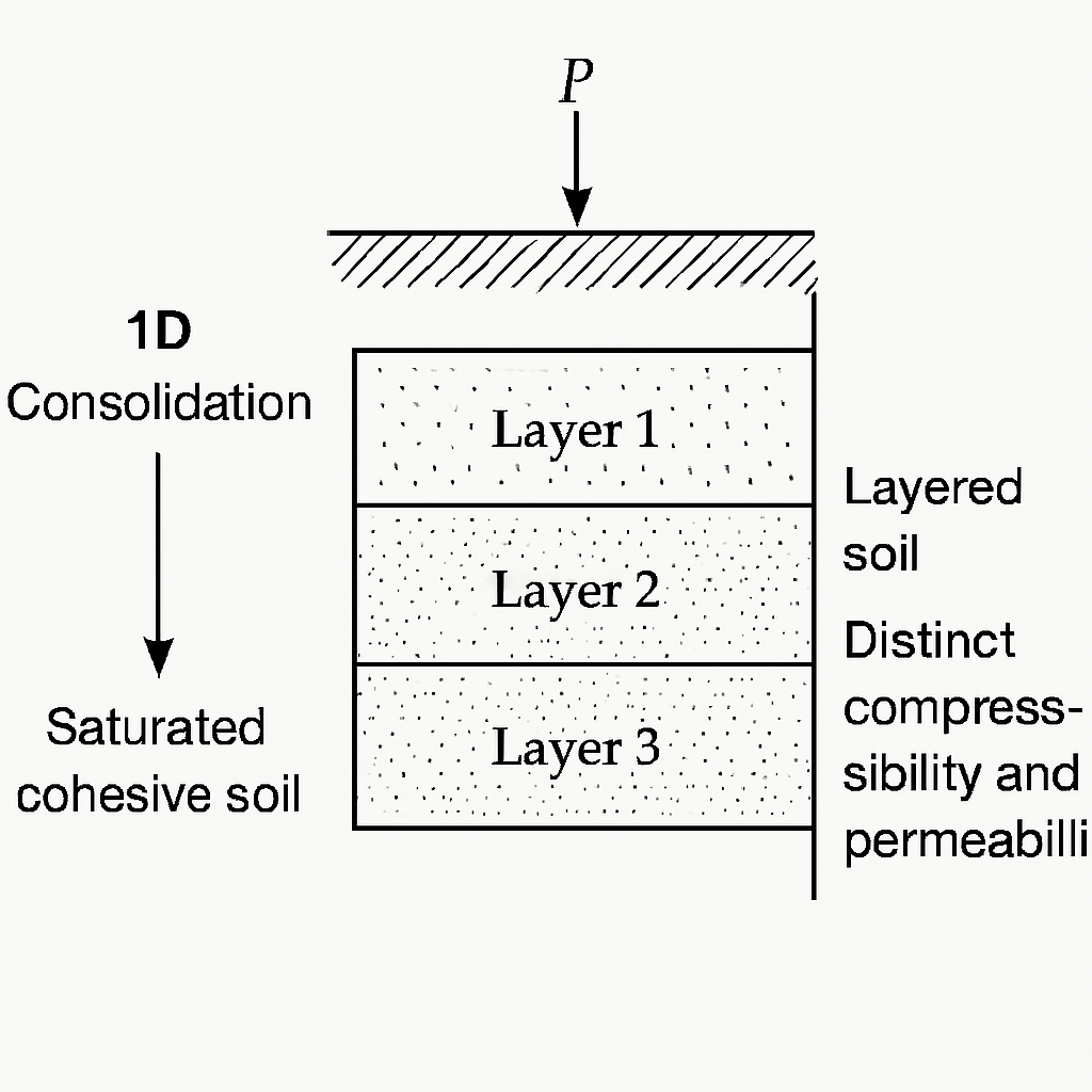
Fig. 20 **Figure 4.7 **: 1D Consolidation Test.#
🧱 Soil Consolidation:#
Soil consolidation is the process by which soil volume decreases over time due to the expulsion of pore water under sustained loading. It primarily occurs in saturated cohesive soils (e.g., clay) and is governed by the gradual transfer of stress from water to soil particles.
When a load (e.g., building, embankment, dam) is applied to saturated soil:
Initially, the load is carried by pore water pressure
Over time, water drains out, and the load is transferred to the soil skeleton
This causes settlement and reduction in void ratio
🧱 1D Consolidation Test – Key Steps per U.S. Standard (ASTM D2435/D4186)#
The 1D Consolidation Test evaluates the compressibility and rate of consolidation of cohesive soils under axial load, as defined by [] (incremental loading method) and [] (continuous loading method). Here’s a summary of the standard measurement steps:
📘 ASTM D2435 – Incremental Loading Procedure []#
Step |
Description |
Notes |
|---|---|---|
1️⃣ |
Prepare soil specimen (typically 20–25 mm thick) |
Saturate with water, trim uniformly |
2️⃣ |
Assemble specimen in consolidation ring |
Ensure drainage top and bottom |
3️⃣ |
Place in load frame and saturate sample |
Record initial height and area |
4️⃣ |
Apply incremental loads (e.g. 12.5, 25, 50, … kPa) |
Typically double per step |
5️⃣ |
Record dial gauge readings over time |
Track deformation at intervals (0.25, 1, 2, 4, 8… mins) |
6️⃣ |
Maintain each load for 24 hours or until deformation rate is negligible |
Use time–deformation curve |
7️⃣ |
Unload incrementally and monitor rebound |
Observe elastic recovery |
8️⃣ |
Oven-dry sample to determine moisture content |
Required for calculating void ratio |
9️⃣ |
Calculate compression index (Cc) and coefficient of consolidation (Cv) |
Use log–strain regression and time factor (Tv) |
🧪 Key Parameters Measured#
Dial Deflection → vertical deformation
Elapsed Time (t) → rate of settlement
Applied Stress (σ) → total vertical load
Specimen Dimensions → area and initial height
Moisture Content → for calculating void ratio and strain
📐 Outputs#
Parameter |
Formula |
Usage |
|---|---|---|
Cc |
\(( C_c = \frac{\Delta e}{\log(\sigma_2/\sigma_1)} \)) |
Compressibility of soil |
Cv |
\(( C_v = \frac{T_v \cdot H^2}{t_{50}} \)) |
Settlement rate prediction |
Strain (%) |
\(( \Delta H / H_0 \times 100 \)) |
Deformation under load |
Void Ratio (e) |
Based on moisture and unit weight |
Required for settlement calculations |
✅ Visual Checklist of Test Steps (ASTM D2435)#
Step |
Task |
Observation Point |
|---|---|---|
1️⃣ |
Prepare saturated, trimmed specimen |
Uniform dimensions; full saturation |
2️⃣ |
Place specimen in ring with porous stones |
No trapped air; drainage enabled |
3️⃣ |
Position assembly in loading frame |
Ensure proper alignment and contact |
4️⃣ |
Attach dial gauge or LVDT |
Zero reading; full-range accessibility |
5️⃣ |
Apply first load increment |
Record initial dial deflection |
6️⃣ |
Capture dial readings over time |
Recommended intervals: |
7️⃣ |
Increase load incrementally |
Typically double each step (e.g., 12.5 → 25 → 50 kPa…) |
8️⃣ |
Monitor rebound on unloading |
Elastic recovery noted |
9️⃣ |
Oven-dry sample for moisture content |
For void ratio and compressibility |
🔟 |
Analyze strain–log(stress), t₅₀, and compute Cc and Cv |
Graphs and regression output |
References#
[]: Standard method for determining one-dimensional consolidation properties of saturated soils using incremental loading. Widely used in geotechnical practice for estimating settlement and compression characteristics of cohesive soils. [ASTM International, 2020]: Standard method using controlled-strain (CRS) loading to evaluate consolidation behavior. Offers faster testing and continuous data acquisition, suitable for advanced lab setups and detailed soil behavior analysis. Both standards are recognized in U.S. geotechnical engineering for characterizing settlement potential and time-rate of consolidation in foundation design.
2. Simulation#
🧱 Summary of the 1D Consolidation Test App (ASTM D2435 Interactive Module)#
An interactive Python app built with ipywidgets that simulates the 1D Consolidation test for soil samples. It allows users to input lab data and automatically computes:
Vertical strain under stepwise loading
Compression Index (Cc) for estimating compressibility
Consolidation Coefficient (Cv) for predicting settlement rate
⚙️ What It Does#
Feature |
Description |
|---|---|
Input dial readings |
Accepts initial/final dial gauge values per load increment |
Computes strain |
Calculates vertical strain (%) from dial compression |
Regression for Cc |
Fits a line to strain vs. log stress for compression index |
Computes Cv |
Uses t₅₀ and specimen height to calculate consolidation rate |
Generates report |
Summarizes data in Markdown with optional plot visualization |
🧮 How to Interpret the Output#
Key Results#
Strain (%): Relative vertical deformation from load
Cc: Compression Index
↳ Higher Cc ⇒ more compressible soil
↳ Used to estimate settlement from effective stress changeCv (m²/s): Coefficient of Consolidation
↳ Larger Cv ⇒ faster dissipation of pore water
↳ Important for evaluating settlement duration and stability
Use in Design#
Cc and Cv are foundational parameters for predicting:
Primary consolidation settlement
Time-dependent deformation
Earthwork and foundation stability over time
import pandas as pd
import numpy as np
import ipywidgets as widgets
from IPython.display import display, Markdown
import matplotlib.pyplot as plt

# 📐 Style
style = {'description_width': '200px'}
layout = widgets.Layout(width='400px')

# 📋 Specimen Parameters
specimen_area = widgets.FloatText(value=0.00785, description='Specimen Area (m²):', style=style, layout=layout)
specimen_height = widgets.FloatText(value=0.025, description='Initial Height (m):', style=style, layout=layout)
load_increment = widgets.FloatText(value=12.5, description='Load Increment (kPa):', style=style, layout=layout)
num_increments = widgets.IntSlider(value=5, min=1, max=12, description='Load Steps:', style=style, layout=layout)
t50_input = widgets.FloatText(value=240, description='t₅₀ Time (min):', style=style, layout=layout)

# 🧪 Atterberg Limits for USCS
LL_input = widgets.FloatText(value=45.0, description='Liquid Limit (LL%)', style=style, layout=layout)
PL_input = widgets.FloatText(value=25.0, description='Plastic Limit (PL%)', style=style, layout=layout)

# 📥 Generate Reading Inputs
def create_reading_inputs(n):
    inputs = []
    for i in range(n):
        d0 = widgets.FloatText(value=0.00, description=f'Trial {i+1} – Dial Initial (mm)', style=style, layout=layout)
        df = widgets.FloatText(value=0.25, description=f'Trial {i+1} – Dial Final (mm)', style=style, layout=layout)
        duration = widgets.FloatText(value=240, description=f'Trial {i+1} – Time (min)', style=style, layout=layout)
        inputs.append((d0, df, duration))
    return inputs

reading_inputs = create_reading_inputs(num_increments.value)

def update_inputs(change):
    global reading_inputs
    reading_inputs = create_reading_inputs(change['new'])
    input_box.children = [
        specimen_area, specimen_height, load_increment, t50_input,
        LL_input, PL_input
    ] + [w for group in reading_inputs for w in group]

num_increments.observe(update_inputs, names='value')

input_box = widgets.VBox([
    specimen_area, specimen_height, load_increment, t50_input,
    LL_input, PL_input
] + [w for group in reading_inputs for w in group])

run_btn = widgets.Button(description='Generate Full Report', layout=widgets.Layout(width='260px'))

# 🧭 USCS Classification Logic
def classify_uscs(ll, pl):
    pi = ll - pl
    if ll < 50:
        if pi < 4:
            return "ML – Low plasticity silt"
        elif pi < 7:
            return "CL or ML – Borderline low plasticity"
        elif pi <= 20:
            return "CL – Lean clay"
        else:
            return "CL – Medium plasticity clay"
    else:
        if pi <= 20:
            return "MH – Elastic silt"
        else:
            return "CH – Fat clay"

# 🧮 Main Logic
def on_run_click(b):
    A = specimen_area.value
    H0 = specimen_height.value
    dP = load_increment.value
    t50 = t50_input.value * 60
    LL = LL_input.value
    PL = PL_input.value
    PI = LL - PL
    classification = classify_uscs(LL, PL)

    rows = []
    cumulative_load = 0

    for i, (d_init, d_final, time) in enumerate(reading_inputs):
        cumulative_load += dP
        d1 = d_init.value / 1000
        d2 = d_final.value / 1000
        strain = (d2 - d1) / H0 if H0 > 0 else 0
        rows.append({
            'Step': i + 1,
            'Applied Stress (kPa)': cumulative_load,
            'Dial Initial (mm)': round(d_init.value, 2),
            'Dial Final (mm)': round(d_final.value, 2),
            'Strain (%)': round(strain * 100, 3),
            'Time (min)': time.value,
            'Log(Stress)': np.log10(max(cumulative_load, 1))
        })

    df = pd.DataFrame(rows)

    # 📊 Report Markdown
    report_md = """

### 🧱 Consolidation Report – ASTM D2435

| Step | Stress (kPa) | Dial Init (mm) | Dial Final (mm) | Strain (%) | Time (min) |
|------|--------------|----------------|------------------|-------------|------------|
"""
    for row in rows:
        report_md += f"| {row['Step']} | {row['Applied Stress (kPa)']} | {row['Dial Initial (mm)']} | {row['Dial Final (mm)']} | {row['Strain (%)']} | {row['Time (min)']} |\n"

    report_md += f"""
#### 📌 Specimen Details
- **Area**: {A:.5f} m²
- **Initial Height**: {H0:.3f} m
- **Load Increment**: {dP:.1f} kPa
- **t₅₀ Time**: {t50 / 60:.1f} min

---
"""

    # 📈 Cc Calculation & Plot
    df_fit = df[df['Applied Stress (kPa)'] >= df['Applied Stress (kPa)'].max() * 0.5]
    if len(df_fit) >= 2:
        x = df_fit['Log(Stress)']
        y = df_fit['Strain (%)']
        slope, intercept = np.polyfit(x, y, 1)
        fit_line = slope * df['Log(Stress)'] + intercept
        Cc = round(slope / 100, 4)

        fig, ax = plt.subplots(figsize=(6, 4))
        ax.plot(df['Log(Stress)'], df['Strain (%)'], 'bo-', label='Measured Strain')
        ax.plot(df['Log(Stress)'], fit_line, 'r--', label='Cc Regression')
        ax.set_xlabel('Log(Stress) [log(kPa)]')
        ax.set_ylabel('Strain (%)')
        ax.set_title('Strain vs. Log(Stress) – Cc Fit')
        ax.grid(True)
        ax.legend()
        plt.show()

        report_md += f"""
### 📊 Compression Index (Cc)

- **Cc** = {Cc:.4f}
- Based on strain–log(σ′) regression for final increments
"""
    else:
        report_md += "⚠️ Insufficient data to compute compression index (Cc).\n"

    # ⏳ Cv Calculation
    Tv = 0.197
    Hdr = H0 / 2
    Cv = (Tv * Hdr ** 2) / t50 if t50 > 0 else 0
    report_md += f"""
### ⏳ Coefficient of Consolidation (Cv)

- **Cv** = {Cv:.6f} m²/s
- Based on t₅₀ = {t50 / 60:.1f} min and Hdr = {Hdr:.3f} m
"""

    # 📘 USCS Output
    report_md += f"""
### 🧭 USCS Classification (Atterberg Limits)

- **Liquid Limit (LL)** = {LL:.1f} %
- **Plastic Limit (PL)** = {PL:.1f} %
- **Plasticity Index (PI)** = {PI:.1f} %
- **USCS Group** = {classification}
"""

    display(Markdown(report_md))

run_btn.on_click(on_run_click)

# 📦 Display Interface
display(widgets.VBox([num_increments, input_box, run_btn]))
3. Self-Assessment#
🧱 1D Consolidation Test – Conceptual, Reflective & Quiz Questions#
🔍 Conceptual Questions#
What does the compression index (Cc) indicate about the compressibility of soil under load?
Why is strain plotted against log of vertical stress in evaluating soil consolidation behavior?
How does the coefficient of consolidation (Cv) influence the rate at which pore water dissipates?
What is the significance of determining the time for 50% consolidation (t₅₀)?
How do specimen geometry and drainage path affect the interpretation of Cv?
💭 Reflective Questions#
While reviewing your test data, which load steps showed nonlinear strain responses—and what might that imply?
What factors in a lab setup could influence the accuracy of dial readings or strain measurements?
If you observed a sudden drop in strain between two stress increments, how would you explain it?
How would you communicate the meaning of Cc and Cv to a field engineer overseeing embankment construction?
What challenges might arise when translating lab-calculated Cv into field-scale predictions?
Theory & Interpretation#
Q1. What is the formula used to calculate the compression index (Cc)?
A. \(( C_c = \Delta e / \log(\sigma_2 / \sigma_1) \)) ✅
B. \(( C_c = \Delta H / H_0 \))
C. \(( C_c = \gamma_w \cdot t / H_0^2 \))
D. \(( C_c = \sigma_2 - \sigma_1 \))
Q2. The time factor (Tv) for 50% consolidation using the square-root method is approximately:
A. 0.5
B. 0.197 ✅
C. 1.0
D. 0.10
Q3. Cv is computed from which variables?
A. Load and compression index
B. Time and specimen diameter
C. Drainage path length and time to 50% consolidation ✅
D. Moisture content and bulk density
Data & Reasoning#
Q4. A higher Cv value generally indicates:
A. Slower water dissipation
B. Faster consolidation rate ✅
C. More clay content
D. Higher shrinkage
Q5. Why is the drainage path taken as H₀/2 in double-drainage setups?
A. Because water exits only one face
B. Because soil drains vertically and horizontally
C. Because both top and bottom surfaces allow drainage ✅
D. Because initial strain is halved
Would you like these embedded into the app as interactive explanations or formatted as a worksheet for learner assessment?