
Chapter 3 Hydraulics: Hydraulic and Hydrologic Routing#
1. Introduction#
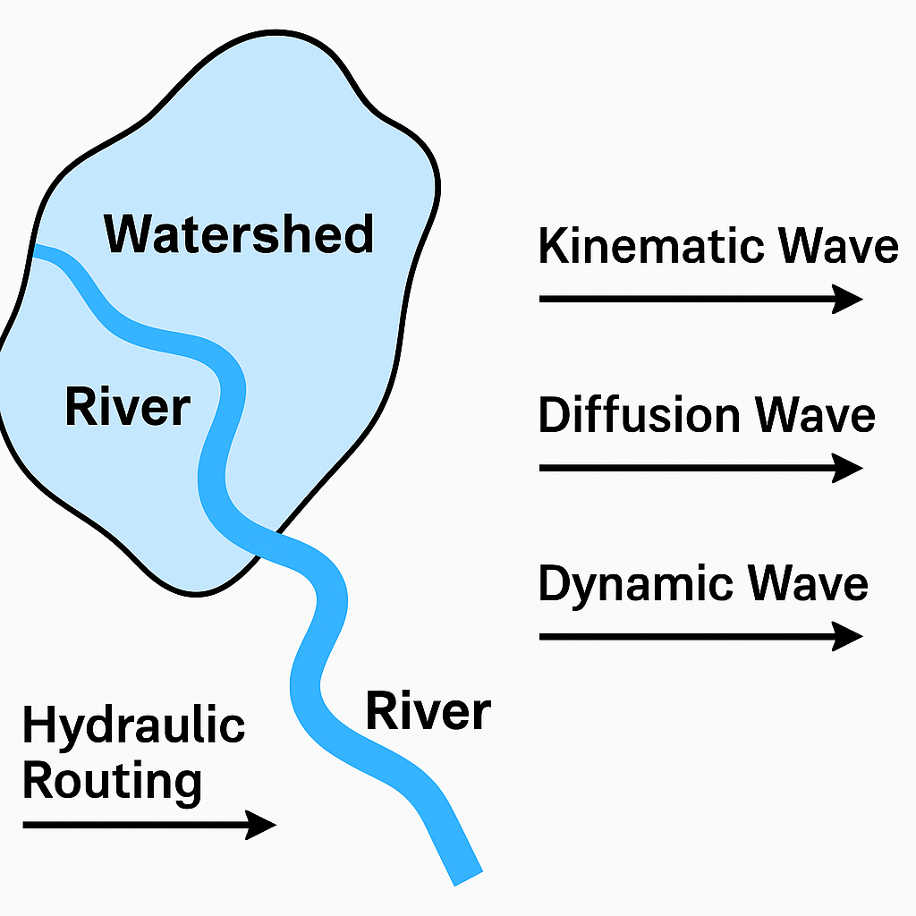
Fig. 7 **Figure 3.3 **: Hydrologic and Hydraulic Routing.#
🌊 Hydraulic Routing – Definition, Types & Importance#
Hydraulic routing is a method used to simulate the movement of water through rivers, channels, or reservoirs by solving the Saint-Venant equations—a set of partial differential equations that describe unsteady open-channel flow. Unlike hydrologic routing (which uses only the continuity equation), hydraulic routing incorporates both mass conservation and momentum conservation, making it more physically accurate.
📘 What Is Hydrologic Routing?#
Hydrologic routing refers to the process of predicting the change in flow rate (discharge) at different points along a channel or reservoir over time, based on upstream inputs.
Unlike hydraulic routing (which uses detailed flow mechanics), hydrologic routing focuses on storage and continuity relationships rather than spatial velocity profiles.🔸 Core Assumptions: - Lumped system (flow treated as a single variable in space); - Based on continuity equation (storage = inflow – outflow)
Commonly uses hydrographs as input/output tools
🧮 Governing Equations#
1. Continuity Equation (Mass Conservation)#
\(( A \)): Cross-sectional area
\(( Q \)): Discharge
\(( x \)): Distance along channel
\(( t \)): Time
\(( q_l \)): Lateral inflow per unit length
2. Momentum Equation#
\(( h \)): Flow depth
\(( g \)): Gravity
\(( S_0 \)): Channel bed slope
\(( S_f \)): Friction slope
\(( v_l \)): Velocity of lateral inflow
🔀 Types of Hydraulic Routing#
1. Kinematic Wave Routing#
Simplifies momentum equation by neglecting pressure and inertial terms.
Assumes: $\( S_f = S_0 \)$
Suitable for steep channels and overland flow.
2. Diffusion Wave Routing#
Retains pressure term but neglects inertial terms.
Equation: $\( \frac{\partial Q}{\partial t} + gA \frac{\partial h}{\partial x} = gA(S_0 - S_f) \)$
Captures backwater effects and mild slopes.
3. Dynamic Wave Routing#
Full Saint-Venant equations.
Captures all flow regimes including subcritical, supercritical, and mixed flows.
Most accurate but computationally intensive.
🌍 Importance in Hydrologic, Hydraulic & Ecohydraulic Studies#
✅ Hydrologic Applications#
Accurate flood forecasting and hydrograph translation
Reservoir and channel design
Watershed modeling and runoff routing
✅ Hydraulic Applications#
Design of culverts, spillways, and energy dissipators
Simulation of flow transitions (e.g., hydraulic jumps)
Urban drainage and stormwater systems
✅ Ecohydraulic Applications#
Modeling habitat suitability for aquatic species
Assessing flow variability and sediment transport
Designing environmental flow regimes
🧪 General Hydraulic Routing Methods#
1. Kinematic Wave Routing#
Simplest method
Assumes friction slope equals bed slope: ( S_f = S_0 )
Ignores pressure and inertial effects
Based on continuity only
2. Diffusion Wave Routing#
Includes pressure term from momentum equation
Neglects inertial acceleration
Handles backwater effects
Suitable for gentle slopes and gradually varied flow
3. Dynamic Wave Routing#
Uses full Saint-Venant equations
Captures all flow regimes (supercritical, subcritical, mixed)
Most physically accurate
Requires numerical methods (e.g., Preissmann scheme, MacCormack)
4. Muskingum Routing (Hydrologic)#
Empirical method based on continuity
Models the storage-discharge relationship
Simpler than hydraulic routing
Often used for river routing in hydrologic models
📊 Comparison Table#
Method |
Governing Equations |
Captures Backwater |
Flow Regimes |
Complexity |
Best Use Case |
|---|---|---|---|---|---|
Kinematic Wave |
Continuity only, ( S_f = S_0 ) |
❌ No |
Supercritical only |
Low |
Overland flow, steep channels |
Diffusion Wave |
Continuity + pressure term |
✅ Yes |
Subcritical |
Medium |
Mild slope rivers, floodplains |
Dynamic Wave |
Full Saint-Venant (continuity + momentum) |
✅ Yes |
All regimes |
High |
Flood modeling, dam breach, urban drainage |
Muskingum (hydrologic) |
Continuity + empirical storage |
❌ No |
Lumped flow |
Low |
River routing in large basins |
🌧️ Hydrologic Routing: Key Equation#
📐 Key Equations#
1. Continuity Equation#
Where:
\(( S \)): storage
\(( I \)): inflow
\(( Q \)): outflow
2. Muskingum Method#
A widely used hydrologic routing technique:
Where:
\(( K \)): storage time constant
\(( X \)): weighting factor (0 to 0.5)
Suitable for river routing
🧭 Why Is Hydrologic Routing Important?#
🔹 Forecasting Floods#
Predicts timing and magnitude of downstream peak discharge
Guides flood warning and mitigation strategies
🔹 Storage Management#
Informs reservoir operations (e.g. drawdown or retention)
Helps plan gate releases and detention schedules
🔹 Infrastructure Design#
Determines flow regime for culverts, bridges, spillways
Evaluates downstream impacts of urban drainage systems
🔹 Simulation & Modeling#
Integral to rainfall-runoff and watershed models (e.g., HEC-HMS, SWMM)
Useful in calibration of hydrologic responses in planning scenarios
🏗️ Application Areas#
Sector |
Use of Hydrologic Routing |
|---|---|
Floodplain Mapping |
Predicts hydrograph shape for risk zones |
Dam & Reservoir Operations |
Guides controlled releases and overflow planning |
Urban Stormwater Systems |
Models detention basins and conveyance networks |
Watershed Management |
Helps quantify upstream land-use impact downstream |
Emergency Response Systems |
Supports evacuation and infrastructure protection |
References#
[Gupta, 2017] Covers both application-driven approach towards hydrologic and hydraulic routing methods (e.g., Muskingum, kinematic wave, and dynamic wave routing). Whereas [Chow et al., 1988] presents routing with a systems-based, conceptual focus, introducing both hydrologic and hydraulic methods.
2. Simulation#
🔍 Hydraulic Routing Simulator Using Muskingum and Kinematic Wave Methods#
An interactive Jupyter Notebook tool for routing a synthetic inflow hydrograph using two widely applied methods:
Muskingum Method (hydraulic routing with storage and attenuation)
Kinematic Wave Method (approximate translation-based routing)
⚙️ How It Works#
1. Inflow Hydrograph Generation#
Creates a Gaussian-shaped inflow hydrograph: $\( I(t) = Q_{\text{peak}} \cdot \exp[-0.4 \cdot (t - t_{\text{peak}})^2] \)$
2. Muskingum Routing Equation#
Updates outflow using weighted contributions: $\( O_t = C_0 I_t + C_1 I_{t-1} + C_2 O_{t-1} \)$ with:
\(( C_0 = \frac{-Kx + 0.5\Delta t}{K - Kx + \Delta t} \))
\(( C_1 = \frac{Kx + 0.5\Delta t}{K - Kx + \Delta t} \))
\(( C_2 = \frac{K - \Delta t}{K - Kx + \Delta t} \))
3. Kinematic Wave Routing Equation#
Approximates outflow using a linear reservoir response: $\( O_t = O_{t-1} + \frac{I_t - O_{t-1}}{k} \)$
🧾 Input Parameters#
Variable |
Description |
|---|---|
|
Total time span (hr) |
|
Maximum inflow rate (m³/s) |
|
Hour of peak inflow |
|
Routing time step (hr) |
|
Muskingum travel time coefficient (hr) |
|
Muskingum weighting factor (0–0.5) |
|
Kinematic storage coefficient (hr) |
📈 Output Interpretation#
Plot Element |
Meaning |
|---|---|
Blue Line |
Inflow hydrograph (reference curve) |
Green Line |
Routed outflow via Muskingum (shows attenuation & lag) |
Red Line |
Kinematic outflow (simpler translation, less attenuation) |
Markdown Summary |
Peak values and lag indicators for all methods |
This tool lets you compare routing responses and visually explore how parameters like K, x, and k impact flow attenuation and timing in open channel systems.
2. Simulation#
import numpy as np
import matplotlib.pyplot as plt
import ipywidgets as widgets
from IPython.display import display, Markdown, clear_output

# --- Generate inflow hydrograph (Gaussian) ---
def generate_inflow(duration=24, peak_flow=100, peak_time=6):
    t = np.arange(0, duration + 1)
    I = peak_flow * np.exp(-0.4 * (t - peak_time)**2)
    return t, I

# --- Muskingum Routing ---
def muskingum(I, K, x, Δt):
    C0 = (-K * x + 0.5 * Δt) / (K - K * x + Δt)
    C1 = (K * x + 0.5 * Δt) / (K - K * x + Δt)
    C2 = (K - Δt) / (K - K * x + Δt)
    O = [I[0]]
    for t in range(1, len(I)):
        O_new = C0 * I[t] + C1 * I[t - 1] + C2 * O[-1]
        O.append(O_new)
    return np.array(O)

# --- Kinematic Wave Routing (linear reservoir approx) ---
def kinematic_wave(I, k_coeff):
    O = [I[0]]
    for t in range(1, len(I)):
        O_new = O[-1] + (I[t] - O[-1]) / k_coeff
        O.append(O_new)
    return np.array(O)

# --- Interactive widgets ---
duration_slider = widgets.IntSlider(value=24, min=12, max=72, description="Duration (hr)")
peakQ_slider = widgets.FloatSlider(value=100, min=10, max=500, step=10, description="Peak Q (m³/s)")
peakT_slider = widgets.IntSlider(value=6, min=1, max=24, description="Peak Time (hr)")
K_slider = widgets.FloatSlider(value=5.0, min=1.0, max=20.0, step=0.1, description="Muskingum K (hr)")
x_slider = widgets.FloatSlider(value=0.3, min=0.0, max=0.5, step=0.05, description="Muskingum x")
k_slider = widgets.FloatSlider(value=3.0, min=0.5, max=10.0, step=0.1, description="Kinematic k")
Δt_slider = widgets.FloatSlider(value=1.0, min=0.1, max=4.0, step=0.1, description="Δt (hr)")
btn = widgets.Button(description="Route Flow")
out = widgets.Output()

def on_click(b):
    with out:
        clear_output()
        t, I = generate_inflow(duration_slider.value, peakQ_slider.value, peakT_slider.value)
        O_musk = muskingum(I, K_slider.value, x_slider.value, Δt_slider.value)
        O_kin = kinematic_wave(I, k_slider.value)

        plt.figure(figsize=(10, 5))
        plt.plot(t, I, label="Inflow", color='blue')
        plt.plot(t, O_musk, label="Muskingum Outflow", color='green')
        plt.plot(t, O_kin, label="Kinematic Outflow", color='red')
        plt.xlabel("Time (hr)")
        plt.ylabel("Flow (m³/s)")
        plt.title("Hydraulic Routing: Muskingum vs. Kinematic Wave")
        plt.legend()
        plt.grid(True)
        plt.show()

        display(Markdown(f"""
        ### ✅ Routing Results
        - **Peak Inflow:** `{max(I):.1f} m³/s`
        - **Muskingum Peak Outflow:** `{max(O_musk):.1f} m³/s` at hr `{np.argmax(O_musk)}`
        - **Kinematic Peak Outflow:** `{max(O_kin):.1f} m³/s` at hr `{np.argmax(O_kin)}`
        - **Attenuation & Lag Visible** – Explore K, x, and k impact
        """))

btn.on_click(on_click)

# --- Display UI ---
display(widgets.VBox([
    widgets.HTML("<h3>🌊 Hydraulic Routing – Muskingum & Kinematic Wave Comparison</h3>"),
    duration_slider, peakQ_slider, peakT_slider,
    Δt_slider, K_slider, x_slider, k_slider,
    btn, out
]))
3. Simulation#
Interactive Storage Routing with User-Selectable Outlet Type#
A Jupyter Notebook tool that models how a detention basin routes an inflow hydrograph through storage and outlet hydraulics. Users can interactively select outlet type: Weir, Orifice, or a combination — and choose between weir styles like Broad-Crested, Sharp-Crested, or V-Notch.
⚙️ How It Works#
Generates a synthetic inflow hydrograph shaped like a Gaussian curve.
Tracks storage volume and depth over time: $\( V_{\text{storage}}^{t} = V^{t-1} + \text{Inflow} \cdot \Delta t - \text{Outflow} \cdot \Delta t \)\( \)\( h = \frac{V_{\text{storage}}}{A} \)$
Calculates outflow based on hydraulic conditions:
Weir Equation: $\( Q = C_w \cdot L_w \cdot H^{1.5} \quad \text{(or } Q = 1.4 \cdot H^{2.5} \text{ for V-notch)} \)$
Orifice Equation: $\( Q = C_o \cdot A_o \cdot \sqrt{2g(H - h_e)} \)$
Plots inflow vs outflow hydrographs and storage volume over time.
🧾 Inputs#
Widget |
Description |
|---|---|
Duration, Δt |
Routing time window and timestep (hr) |
Peak Flow, Peak Time |
Defines shape of inflow hydrograph |
Storage Area (m²) |
Basin surface area for depth calculation |
Outlet Type |
Choose Weir, Orifice, or Weir + Orifice |
Weir Type |
Broad-Crested, Sharp-Crested, or V-Notch |
Cw, Lw |
Weir coefficient and crest length |
Co, Ao, he |
Orifice coefficient, area, and elevation |
📈 Output Interpretation#
Hydrograph plot:
Blue: Inflow
Green: Routed outflow, shaped by outlet hydraulics
Storage plot:
Purple curve shows how basin volume builds and drains
Output Metric |
Meaning |
|---|---|
Peak Inflow/Outflow |
Maximum flow rates in each curve |
Storage Volume |
Shows how much water is temporarily held |
Depth (h) |
Indicates water level relative to outlet |
Routing Lag |
Delay between inflow and outflow peak |
Use this tool to explore how outlet design affects flow attenuation, peak shaving, and detention performance in stormwater systems.
# 📘 Interactive Storage Routing – User-Selectable Outlet Type (Weir / Orifice)

import numpy as np
import matplotlib.pyplot as plt
import ipywidgets as widgets
from IPython.display import display, Markdown, clear_output

# --- Synthetic inflow hydrograph ---
def generate_inflow(duration, peakflow, peaktime):
    t = np.arange(0, duration + 1)
    I = peakflow * np.exp(-0.4 * (t - peaktime)**2)
    return t, I

# --- Outlet flow equations ---
def weir_flow(H, weir_type, Cw, Lw):
    if H <= 0: return 0.0
    if weir_type == "Broad-Crested":
        return Cw * Lw * H**1.5
    elif weir_type == "Sharp-Crested":
        return Cw * Lw * H**1.5
    elif weir_type == "V-Notch":
        angle = 90  # degrees; can be parameterized later
        return 1.4 * H**2.5  # Approximate V-notch formula
    else:
        return Cw * Lw * H**1.5  # default

def orifice_flow(H, Co, Ao, he=0.6):
    return Co * Ao * np.sqrt(2 * 9.81 * max(H - he, 0)) if H > he else 0.0

def outlet_flow(H, outlet_mode, weir_type, Cw, Lw, Co, Ao, he):
    if outlet_mode == "Weir":
        return weir_flow(H, weir_type, Cw, Lw)
    elif outlet_mode == "Orifice":
        return orifice_flow(H, Co, Ao, he)
    elif outlet_mode == "Weir + Orifice":
        return weir_flow(H, weir_type, Cw, Lw) + orifice_flow(H, Co, Ao, he)
    else:
        return 0.0

# --- Storage routing ---
def storage_routing(I, Δt, A, outlet_mode, weir_type, Cw, Lw, Co, Ao, he):
    S, O, H = [0.0], [0.0], [0.0]
    for i in range(1, len(I)):
        Vin = I[i] * Δt * 3600
        Vout = O[-1] * Δt * 3600
        Snew = max(0, S[-1] + Vin - Vout)
        Hnew = Snew / A
        Onew = outlet_flow(Hnew, outlet_mode, weir_type, Cw, Lw, Co, Ao, he)
        S.append(Snew)
        H.append(Hnew)
        O.append(Onew)
    return np.array(O), np.array(S), np.array(H)

# --- Widgets ---
duration = widgets.IntSlider(value=24, min=6, max=72, description="Duration (hr)")
peakQ = widgets.FloatSlider(value=100, min=10, max=500, step=10, description="Peak Flow")
peakT = widgets.IntSlider(value=6, min=1, max=24, description="Peak Time (hr)")
Δt = widgets.FloatSlider(value=1.0, min=0.1, max=4.0, step=0.1, description="Δt (hr)")
area = widgets.FloatText(value=1000, description="Storage Area (m²)")

outlet_mode = widgets.Dropdown(options=["Weir", "Orifice", "Weir + Orifice"], value="Weir", description="Outlet Type")
weir_type = widgets.Dropdown(options=["Broad-Crested", "Sharp-Crested", "V-Notch"], value="Broad-Crested", description="Weir Type")

Cw = widgets.FloatText(value=1.7, description="Weir C")
Lw = widgets.FloatText(value=5.0, description="Weir Length (m)")

Co = widgets.FloatText(value=0.6, description="Orifice Coef")
Ao = widgets.FloatText(value=0.5, description="Orifice Area (m²)")
he = widgets.FloatText(value=0.6, description="Orifice Elev (m)")

btn = widgets.Button(description="Run Routing")
out = widgets.Output()

def on_click(b):
    with out:
        clear_output()
        T, I = generate_inflow(duration.value, peakQ.value, peakT.value)
        O, S, H = storage_routing(
            I, Δt.value, area.value,
            outlet_mode.value, weir_type.value,
            Cw.value, Lw.value,
            Co.value, Ao.value, he.value
        )

        fig, axs = plt.subplots(2, 1, figsize=(10, 8))
        axs[0].plot(T, I, label="Inflow", color='blue')
        axs[0].plot(T, O, label="Outflow", color='green')
        axs[0].set_ylabel("Flow (m³/s)")
        axs[0].set_title(f"Hydrograph Routing ({outlet_mode.value})")
        axs[0].legend(); axs[0].grid(True)

        axs[1].plot(T, S, label="Storage Volume", color='purple')
        axs[1].set_ylabel("Volume (m³)")
        axs[1].set_xlabel("Time (hr)")
        axs[1].set_title("Storage Volume Over Time")
        axs[1].grid(True)

        plt.tight_layout(); plt.show()

        display(Markdown(f"""
        ### ✅ Routing Summary
        - Peak Inflow: `{max(I):.1f} m³/s` at `{np.argmax(I)} hr`
        - Peak Outflow: `{max(O):.1f} m³/s` at `{np.argmax(O)} hr`
        - Max Storage: `{max(S):,.1f} m³` | Max Depth: `{max(H):.2f} m`
        - Outlet Type: `{outlet_mode.value}` | Weir Type: `{weir_type.value}`
        """))

btn.on_click(on_click)

# --- Display UI ---
display(widgets.VBox([
    widgets.HTML("<h3>🌊 Storage Routing with Selectable Outlet Type</h3>"),
    duration, peakQ, peakT, Δt, area,
    outlet_mode, weir_type,
    widgets.HBox([Cw, Lw]),
    widgets.HBox([Co, Ao, he]),
    btn, out
]))
4. Self-Assessment#
💧 Hydrologic Routing#
Have you ever encountered a situation where hydrologic routing underestimated peak discharge? What factors might have led to this?
When teaching hydrologic routing, how do you explain the relevance of lumped vs distributed modeling?
How do parameter choices like (K) and (X) in the Muskingum method influence how learners interpret flow attenuation?
🌊 Hydraulic Routing#
How do you decide whether a hydraulic routing model is worth the extra computational effort compared to hydrologic routing?
Reflect on a routing case where spatial velocity profiles were critical—what modeling techniques helped you capture that complexity?
Have you considered integrating momentum-based routing into educational modules? What challenges have you faced?
📘 Conceptual Questions#
💧 Hydrologic Routing#
What are the key assumptions behind the Muskingum method?
How does flow storage in hydrologic routing differ from dynamic storage in hydraulic routing?
Explain why the continuity equation is central to all hydrologic routing methods.
🌊 Hydraulic Routing#
What distinguishes kinematic wave routing from full dynamic wave routing?
Why are momentum and inertial terms retained in Saint-Venant equations but dropped in simpler routing models?
How does flow regime (e.g., subcritical vs supercritical) influence numerical stability in hydraulic routing?
🧪 Quiz Questions#
💧 Hydrologic Routing#
Q1. Hydrologic routing models primarily rely on which equation?
A. Bernoulli equation
B. Continuity equation ✅
C. Energy equation
D. Manning’s equation
Q2. In Muskingum routing, the parameter ( X ):
A. Controls the amount of lateral inflow
B. Represents a velocity head factor
C. Weights the influence of inflow in determining outflow ✅
D. Must always be equal to 1
🌊 Hydraulic Routing#
Q3. Hydraulic routing differs from hydrologic routing by incorporating:
A. Lumped flow parameters
B. Cross-sectional area only
C. Momentum equation and wave celerity ✅
D. Rainfall data directly
Q4. The Saint-Venant equations consist of:
A. One continuity equation only
B. Continuity and momentum equations ✅
C. Energy and pressure equations
D. Manning’s and velocity equations
Q5. Kinematic wave routing assumes:
A. Uniform velocity distribution
B. Negligible inertial forces ✅
C. Backwater effects are significant
D. Reservoir storage must be modeled