
Chapter 2 Hydrology: SpatioTemporal Rainfall Disaggregation#
1. Introduction#
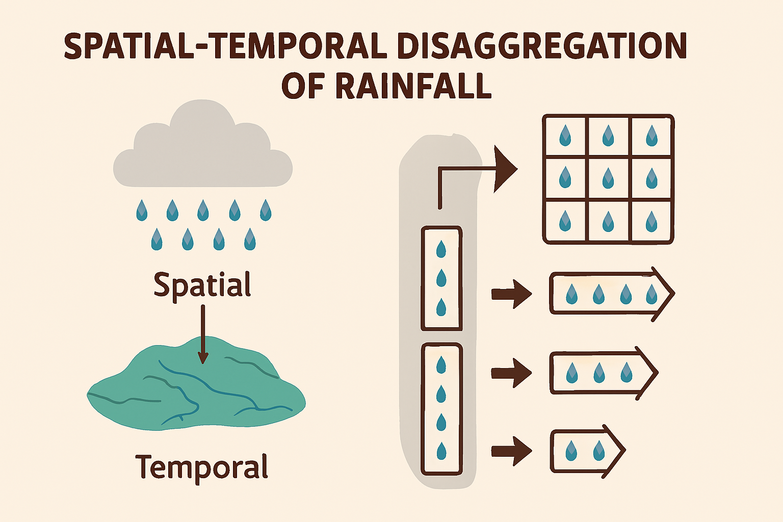
Fig. 1 **Figure 2.0 **: Spatio-Temporal Disaggregation of Rainfall.#
🌧️ Rainfall Disaggregation in Time and Space#
📌 Definition#
Rainfall disaggregation is the process of breaking down coarse-resolution precipitation data into finer temporal and spatial scales.
Temporal disaggregation: Converts daily or monthly rainfall into hourly or minute-level data.
Spatial disaggregation: Allocates rainfall amounts across different spatial units (e.g., catchments, grids).
❓ Why Is Disaggregation Necessary?#
Disaggregation is essential for:
Hydrological modeling: Accurate runoff and flood prediction.
Urban drainage design: Systems respond to short-duration rainfall.
Climate impact studies: Downscaling coarse climate data.
Data scarcity: Generates high-resolution data from limited observations.
⏱️ Temporal Disaggregation Methods#
Method |
Description |
Use Case |
|---|---|---|
Method of Fragments |
Uses historical high-resolution data to split daily totals |
Simple and widely used |
Multiplicative Cascade |
Breaks rainfall into smaller intervals using scaling laws |
Preserves variability |
Poisson Cluster Models |
Simulates rainfall as clusters of events |
Stochastic rainfall generation |
Artificial Neural Networks (ANNs) |
Learns patterns from data to generate sub-daily rainfall |
Data-driven and adaptive |
Generative Adversarial Networks (GANs) |
Learns spatial-temporal patterns from radar data |
Advanced machine learning |
🌍 Spatial Disaggregation Methods#
Method |
Description |
Use Case |
|---|---|---|
Inverse Distance Weighting (IDW) |
Interpolates rainfall based on proximity |
Simple spatial interpolation |
Kriging |
Geostatistical method using spatial correlation |
Accurate but computationally intensive |
Copula-based Models |
Uses joint distributions to simulate spatial rainfall |
Preserves spatial dependence |
Gaussian Markov Random Fields (GMRF) |
Models rainfall as latent Gaussian fields |
Efficient for gridded data |
🌧️ Importance of Rainfall Disaggregation#
Rainfall disaggregation—both in time and space—is essential for accurate hydrological analysis, infrastructure design, and climate adaptation.
⏱️ Temporal Disaggregation#
Temporal disaggregation breaks down daily or monthly rainfall into finer intervals (e.g., hourly or minute-level). Its importance includes:
Hydrological Modeling Accuracy
Captures short-duration, high-intensity rainfall events that drive runoff and erosion.Flood Prediction
Enables simulation of flood peaks, especially in small catchments.Urban Drainage Design
Sub-daily data are critical for designing stormwater systems that respond quickly to rainfall.Climate Change Adaptation
Translates coarse climate model outputs into actionable local-scale data.Water Quality Modeling
Intensity-dependent processes like sediment transport require fine temporal resolution.
🌍 Spatial Disaggregation#
Spatial disaggregation distributes rainfall across different geographic units. Its importance includes:
Catchment-Scale Hydrology
Reflects spatial variability in rainfall, improving runoff and flood estimates.Flood Risk Assessment
Enhances simulation of flood routing, peak flows, and inundation extents.Infrastructure Planning
Critical for designing dams, reservoirs, and levees under extreme rainfall scenarios.Data Scarcity Compensation
Generates localized rainfall patterns from coarse-resolution data.Climate Model Downscaling
Bridges the gap between global climate models and local hydrological applications.
🧠 Combined Impact#
Spatial and temporal disaggregation together:
Enable continuous simulation of rainfall-runoff processes.
Improve extreme event modeling (e.g., PMP and PMF).
Support multi-site analysis for regional water resource planning.
Enhance resilience planning under climate uncertainty.
⚠️ Without disaggregation, hydrological models risk oversimplifying rainfall inputs, leading to poor predictions and unsafe infrastructure designs.
🌧️ PMP and PMF Definitions#
📘 Probable Maximum Precipitation (PMP)#
Definition: The greatest depth of precipitation for a given duration that is physically possible over a particular area.
Use: Design of critical infrastructure (e.g., dams, nuclear plants).
📘 Probable Maximum Flood (PMF)#
Definition: The flood resulting from PMP under worst-case hydrological conditions.
Use: Safety assessment for extreme flood events.
🗺️ Spatial Disaggregation of PMP and PMF#
🧭 PMP Spatial Disaggregation [Hansen et al., 1982].#
Objective: Distribute PMP across a basin or catchment.
Methods:
Isohyetal mapping
Storm transposition and maximization
Radar-based spatial analysis
Hydrometeorological reports
🌊 PMF Spatial Disaggregation#
Objective: Simulate flood hydrographs across sub-basins.
Methods:
Unit hydrograph modeling
Reservoir and channel routing
Monte Carlo simulations
Sensitivity analysis of antecedent conditions
⚠️ Ensure volume consistency and reflect topographic and meteorological variability.
Foundational Literature#
[] is widely recognized as a pioneering study in the United States for estimating Probable Maximum Precipitation (PMP) and, by extension, Probable Maximum Flood (PMF). The method introduced a statistical approach using envelope curves derived from thousands of rainfall records, which became a standard for PMP estimation endorsed by agencies like the World Meteorological Organization (WMO). While Hershfield’s method does not explicitly model storm dynamics or spatial rainfall fields, it laid the groundwork for later spatio-temporal disaggregation techniques by establishing statistical bounds and regional variability in extreme precipitation. [] World Meteorological Organization (WMO) Manual on Estimation of Probable Maximum Precipitation (WMO-No. 1045) is the most foundational and globally recognized reference for PMP and PMF estimation. Provides standardized procedures for estimating Probable Maximum Precipitation (PMP) and Probable Maximum Flood (PMF), and covers storm transposition, moisture maximization, and spatial distribution techniques. The manual includes regional applications from China, USA, Australia, and India.
Rainfall Disaggregation Using Dimensionless Hyetographs#
This interactive model generates sub-hourly rainfall time series from a given total storm depth and duration, using selected dimensionless hyetograph methods. It is commonly used in hydrologic modeling to prepare rainfall inputs for runoff simulations, flood analysis, and stormwater design.
Mathematical Formulation#
Let:
\(( D \)) = total rainfall depth (mm)
\(( T \)) = total storm duration (hr)
\(( \Delta t \)) = time interval (min)
\(( N = \frac{T \times 60}{\Delta t} \)) = number of time steps
\(( f_i \)) = normalized intensity at time step \(( i \))
\(( R_i = D \cdot f_i \)) = rainfall depth at time step \(( i \))
The model computes: $\( \sum_{i=1}^{N} f_i = 1 \quad \Rightarrow \quad R_i = D \cdot f_i \)$
Available Distribution Methods#
1. Triangular Distribution#
A simple peak-centered or skewed distribution: $\( f(t) = \begin{cases} \frac{t}{p}, & t \leq p \\ \frac{1 - t}{1 - p}, & t > p \end{cases} \)$ Where:
\(( t \in [0, 1] \)) is normalized time
\(( p \in (0, 1) \)) is the peak ratio (time of peak intensity)
2. SCS Type II Distribution#
Approximated using a skewed beta-like shape: $\( f(t) = 16 \cdot t^2 \cdot (1 - t)^2 \)$ This mimics the Soil Conservation Service Type II storm used in TR-55 and HEC-HMS.
3. Uniform Distribution#
Assumes constant intensity: $\( f(t) = \frac{1}{N} \)$
Applications#
Hydrologic modeling (e.g., Rational Method, HEC-HMS, SWMM)
Stormwater design (e.g., detention sizing, peak flow estimation)
Flood risk analysis
Synthetic storm generation for sensitivity testing
Limitations and Challenges#
Simplified intensity profiles may not reflect real storm variability
No spatial variation — assumes uniform rainfall over the catchment
No antecedent moisture or infiltration effects
Peak ratio tuning may require calibration to match observed data
SCS approximation is not exact — lacks regional calibration
Tips for Use#
Use Triangular for exploratory or conceptual modeling
Use SCS Type II for regulatory or design compliance
Use Uniform for baseline or control comparisons
Adjust interval and duration to match model resolution and catchment response time
References#
U.S. Soil Conservation Service (1986). Urban Hydrology for Small Watersheds (TR-55)
Chow, V.T., Maidment, D.R., Mays, L.W. (1988). Applied Hydrology
Rossman, L.A. (2010). Storm Water Management Model (SWMM) User’s Manual
Applications of Disaggregated Rainfall in Hydrologic Analysis#
Disaggregated rainfall — rainfall broken into fine time intervals — is essential for dynamic hydrologic modeling. It allows engineers and scientists to simulate how rainfall intensity and timing affect runoff, infiltration, flooding, and infrastructure performance.
Key Applications#
1. Runoff Modeling#
Disaggregated rainfall is used to generate time-varying runoff in models like:
Rational Method: Peak runoff ( Q = CiA ) depends on rainfall intensity ( i ) over the time of concentration.
HEC-HMS, SWMM: Use rainfall time series to produce hydrographs showing flow over time.
2. Flood Routing#
Inflow hydrographs derived from disaggregated rainfall are routed through:
Reservoirs (e.g., level pool routing)
Channels (e.g., Muskingum method)
This helps simulate lag, attenuation, and peak timing of flood waves.
3. Stormwater Infrastructure Design#
Designing detention basins, culverts, and storm sewers requires:
Estimating peak inflow rate
Calculating required storage volume
Evaluating duration of overflow events
Disaggregated rainfall provides the temporal detail needed for these calculations.
4. Infiltration and Soil Moisture Modeling#
Rainfall intensity affects infiltration in models like:
Green-Ampt
Horton
Disaggregated rainfall helps simulate:
Ponding
Saturation
Excess runoff generation
5. Erosion and Sediment Transport#
High-intensity rainfall drives:
Soil detachment
Sediment yield
Used in models like:
WEPP
SWAT
Disaggregated rainfall identifies erosive bursts and transport thresholds.
📊 Example Workflow#
Input: Total rainfall depth = 50 mm, duration = 3 hours
Disaggregation: Break into 10-minute intervals using a triangular or SCS distribution
Hydrologic Model: Use rainfall time series in SWMM to simulate urban runoff
Output: Hydrograph showing peak flow at 1.2 hours, total runoff volume = 35 mm
Design Decision: Size detention basin to handle peak flow and store excess volume
Why It Matters#
Temporal resolution affects the accuracy of peak flow estimates
Design storms must reflect realistic rainfall patterns
Regulatory compliance often requires specific distributions (e.g., SCS Type II)
2. Simulation#
# 📌 Run this cell in a Jupyter Notebook
import numpy as np
import matplotlib.pyplot as plt
import ipywidgets as widgets
from IPython.display import display, clear_output

# 📐 Dimensionless hyetograph generators
def triangular_distribution(n_steps, peak_ratio):
    t = np.linspace(0, 1, n_steps)
    dist = np.where(t <= peak_ratio,
                    t / peak_ratio,
                    (1 - t) / (1 - peak_ratio))
    dist = np.maximum(dist, 0)
    return dist / dist.sum()

def scs_type_ii_distribution(n_steps):
    # Approximate SCS Type II using a skewed beta-like shape
    t = np.linspace(0, 1, n_steps)
    dist = 16 * t**2 * (1 - t)**2  # bell-shaped, peak near center
    return dist / dist.sum()

def uniform_distribution(n_steps):
    return np.ones(n_steps) / n_steps

# 📊 Disaggregation function
def disaggregate_rainfall(total_depth, duration_hr, interval_min, peak_ratio, method):
    n_steps = int((duration_hr * 60) / interval_min)

    # Select method
    if method == 'Triangular':
        distribution = triangular_distribution(n_steps, peak_ratio)
    elif method == 'SCS Type II':
        distribution = scs_type_ii_distribution(n_steps)
    elif method == 'Uniform':
        distribution = uniform_distribution(n_steps)
    else:
        raise ValueError("Unknown method selected.")

    rainfall_series = total_depth * distribution
    time_series = np.linspace(0, duration_hr, n_steps)

    # Plot
    plt.figure(figsize=(10, 5))
    plt.bar(time_series, rainfall_series, width=interval_min / 60, color='dodgerblue', edgecolor='black')
    plt.xlabel('Time (hours)')
    plt.ylabel('Rainfall (mm)')
    plt.title(f'{method} Rainfall Distribution\nTotal Depth = {total_depth:.1f} mm, Duration = {duration_hr:.1f} hr')
    plt.grid(True)
    plt.tight_layout()
    plt.show()

    return time_series, rainfall_series

# 🎚️ Interactive controls
depth_slider = widgets.FloatSlider(value=50.0, min=10.0, max=200.0, step=5.0, description='Total Rainfall (mm)')
duration_slider = widgets.FloatSlider(value=3.0, min=0.5, max=12.0, step=0.5, description='Storm Duration (hr)')
interval_slider = widgets.IntSlider(value=10, min=5, max=60, step=5, description='Interval (min)')
peak_slider = widgets.FloatSlider(value=0.4, min=0.1, max=0.9, step=0.05, description='Peak Ratio')
method_dropdown = widgets.Dropdown(
    options=['Triangular', 'SCS Type II', 'Uniform'],
    value='Triangular',
    description='Method'
)

# 🔄 Display interactive plot
interactive_plot = widgets.interactive(
    disaggregate_rainfall,
    total_depth=depth_slider,
    duration_hr=duration_slider,
    interval_min=interval_slider,
    peak_ratio=peak_slider,
    method=method_dropdown
)

display(interactive_plot)
3. Introduction#
Spatial Rainfall Distribution Model#
This interactive tool simulates the spatial variation of rainfall intensity across a 2D domain, such as a watershed or urban catchment. It helps visualize how rainfall intensity changes with distance from the storm center, using different distribution methods.
Mathematical Formulation#
Let:
\(( R(x, y) \)) = distance from storm center to point ( (x, y) )
\(( P \)) = peak rainfall intensity at the storm center (mm)
\(( r \)) = storm radius or decay scale (km)
1. Gaussian Distribution#
2. Exponential Distribution#
3. Uniform Distribution#
Interactive Controls#
Parameter |
Description |
|---|---|
|
Size of the spatial domain |
|
Number of grid points (controls detail) |
|
Maximum intensity at storm center |
|
Controls decay rate of rainfall |
|
Location of storm center |
|
Distribution type (Gaussian, Exponential, Uniform) |
Applications#
Watershed modeling: Simulate non-uniform rainfall over large basins
Urban hydrology: Assess localized flooding from intense cells
Flood forecasting: Visualize the spatial extent of rainfall input
Design storms: Create synthetic rainfall fields for infrastructure testing
Limitations#
Assumes radial symmetry around storm center
No temporal variation — purely spatial snapshot
Does not account for terrain effects, wind drift, or storm movement
Idealized distributions may differ from observed radar data
Use Cases#
Combine with temporal disaggregation to simulate full spatiotemporal storms
Overlay with watershed boundaries to compute spatially weighted rainfall
Use as input for distributed hydrologic models (e.g., SWAT, GSSHA)
4. Simulation#
# 📌 Run this cell in a Jupyter Notebook
import numpy as np
import matplotlib.pyplot as plt
import ipywidgets as widgets
from IPython.display import display, clear_output

# 📐 Spatial rainfall distribution function
def generate_spatial_rainfall(grid_size_km, resolution, peak_mm, radius_km, center_x, center_y, method):
    clear_output(wait=True)

    # Grid setup
    x = np.linspace(0, grid_size_km, resolution)
    y = np.linspace(0, grid_size_km, resolution)
    X, Y = np.meshgrid(x, y)

    # Distance from storm center
    R = np.sqrt((X - center_x)**2 + (Y - center_y)**2)

    # Distribution methods
    if method == 'Gaussian':
        rainfall = peak_mm * np.exp(- (R**2) / (2 * radius_km**2))
    elif method == 'Exponential':
        rainfall = peak_mm * np.exp(- R / radius_km)
    elif method == 'Uniform':
        rainfall = np.full_like(R, peak_mm)
    else:
        raise ValueError("Unknown method selected.")

    # Plot
    plt.figure(figsize=(8, 6))
    contour = plt.contourf(X, Y, rainfall, levels=50, cmap='Blues')
    plt.colorbar(contour, label='Rainfall (mm)')
    plt.xlabel('X Distance (km)')
    plt.ylabel('Y Distance (km)')
    plt.title(f'Spatial Rainfall Distribution ({method})\nPeak = {peak_mm:.1f} mm, Radius = {radius_km:.1f} km')
    plt.scatter(center_x, center_y, color='red', label='Storm Center')
    plt.legend()
    plt.grid(True)
    plt.tight_layout()
    plt.show()

# 🎚️ Interactive controls
grid_slider = widgets.FloatSlider(value=10.0, min=5.0, max=50.0, step=1.0, description='Grid Size (km)')
resolution_slider = widgets.IntSlider(value=100, min=50, max=300, step=25, description='Resolution')
peak_slider = widgets.FloatSlider(value=50.0, min=10.0, max=200.0, step=5.0, description='Peak Rainfall (mm)')
radius_slider = widgets.FloatSlider(value=3.0, min=0.5, max=10.0, step=0.5, description='Storm Radius (km)')
center_x_slider = widgets.FloatSlider(value=5.0, min=0.0, max=50.0, step=0.5, description='Center X (km)')
center_y_slider = widgets.FloatSlider(value=5.0, min=0.0, max=50.0, step=0.5, description='Center Y (km)')
method_dropdown = widgets.Dropdown(
    options=['Gaussian', 'Exponential', 'Uniform'],
    value='Gaussian',
    description='Method'
)

# 🔄 Display interactive plot
interactive_plot = widgets.interactive(
    generate_spatial_rainfall,
    grid_size_km=grid_slider,
    resolution=resolution_slider,
    peak_mm=peak_slider,
    radius_km=radius_slider,
    center_x=center_x_slider,
    center_y=center_y_slider,
    method=method_dropdown
)

display(interactive_plot)
# 📌 Run this cell in a Jupyter Notebook
import numpy as np
import matplotlib.pyplot as plt
import ipywidgets as widgets
from IPython.display import display, clear_output

# 📐 Step 1: Estimate PMP based on location and duration
def estimate_pmp(lat, lon, duration_hr):
    """
    Simplified empirical PMP estimator.
    Real-world use should rely on NOAA HMR or regional PMP datasets.
    """
    base_pmp = 100 + 2 * (30 - abs(lat))  # latitude effect
    coastal_boost = 50 if abs(lon) < 90 else 0  # crude coastal proximity
    duration_factor = np.sqrt(duration_hr)
    pmp_mm = (base_pmp + coastal_boost) * duration_factor
    return round(pmp_mm, 1)

# 📐 Step 2: Generate spatial distribution of PMP
def generate_pmp_distribution(grid_size_km, resolution, pmp_peak_mm, storm_radius_km, center_x, center_y):
    x = np.linspace(0, grid_size_km, resolution)
    y = np.linspace(0, grid_size_km, resolution)
    X, Y = np.meshgrid(x, y)
    R = np.sqrt((X - center_x)**2 + (Y - center_y)**2)
    PMP = pmp_peak_mm * np.exp(- (R**2) / (2 * storm_radius_km**2))
    return X, Y, PMP

# 📊 Combined interactive function
def estimate_and_plot_pmp(lat, lon, duration_hr, grid_size_km, resolution, storm_radius_km, center_x, center_y):
    clear_output(wait=True)

    # Step 1: Estimate PMP
    pmp_peak_mm = estimate_pmp(lat, lon, duration_hr)

    # Step 2: Generate spatial field
    X, Y, PMP = generate_pmp_distribution(grid_size_km, resolution, pmp_peak_mm, storm_radius_km, center_x, center_y)

    # Display info
    print(f"📍 Location: Latitude {lat:.2f}°, Longitude {lon:.2f}°")
    print(f"🕒 Duration: {duration_hr:.1f} hours")
    print(f"🌧️ Estimated PMP Peak: {pmp_peak_mm:.1f} mm")

    # Plot
    plt.figure(figsize=(8, 6))
    contour = plt.contourf(X, Y, PMP, levels=50, cmap='Purples')
    plt.colorbar(contour, label='PMP (mm)')
    plt.xlabel('X Distance (km)')
    plt.ylabel('Y Distance (km)')
    plt.title(f'Spatial Distribution of PMP\nPeak = {pmp_peak_mm:.1f} mm, Radius = {storm_radius_km:.1f} km')
    plt.scatter(center_x, center_y, color='red', label='Storm Center')
    plt.legend()
    plt.grid(True)
    plt.tight_layout()
    plt.show()

# 🎚️ Interactive controls
lat_slider = widgets.FloatSlider(value=30.0, min=-60.0, max=60.0, step=1.0, description='Latitude (°)')
lon_slider = widgets.FloatSlider(value=-90.0, min=-180.0, max=180.0, step=1.0, description='Longitude (°)')
duration_slider = widgets.FloatSlider(value=6.0, min=1.0, max=72.0, step=1.0, description='Duration (hr)')
grid_slider = widgets.FloatSlider(value=20.0, min=10.0, max=100.0, step=5.0, description='Grid Size (km)')
resolution_slider = widgets.IntSlider(value=100, min=50, max=300, step=25, description='Resolution')
radius_slider = widgets.FloatSlider(value=10.0, min=2.0, max=30.0, step=1.0, description='Storm Radius (km)')
center_x_slider = widgets.FloatSlider(value=10.0, min=0.0, max=100.0, step=1.0, description='Center X (km)')
center_y_slider = widgets.FloatSlider(value=10.0, min=0.0, max=100.0, step=1.0, description='Center Y (km)')

# 🔄 Display interactive plot
interactive_plot = widgets.interactive(
    estimate_and_plot_pmp,
    lat=lat_slider,
    lon=lon_slider,
    duration_hr=duration_slider,
    grid_size_km=grid_slider,
    resolution=resolution_slider,
    storm_radius_km=radius_slider,
    center_x=center_x_slider,
    center_y=center_y_slider
)

display(interactive_plot)
5. Introduction#
Probable Maximum Flood (PMF) Estimation Model#
This interactive tool estimates the Probable Maximum Flood (PMF) volume for a given location using a simplified conceptual approach. PMF represents the largest flood that could conceivably occur at a location, based on the most severe combination of meteorological and hydrologic conditions.
Methodology Overview#
The model follows a two-step process:
1. Estimate Probable Maximum Precipitation (PMP)#
Based on:
Latitude and longitude (to simulate climatic variation)
Storm duration (longer storms yield more precipitation)
A simplified empirical formula is used: $\( \text{PMP} = \left[100 + 2 \cdot (30 - |\text{latitude}|) + \text{coastal boost}\right] \cdot \sqrt{\text{duration (hr)}} \)$ Where:
Coastal boost = 50 mm if longitude suggests proximity to coast (|lon| < 90°)
2. Estimate PMF Volume Using a Runoff Model#
A Rational-like formula is applied: $\( \text{PMF Volume} = C \cdot P \cdot A \)$ Where:
( C ) = runoff coefficient (0–1)
( P ) = PMP depth (converted to meters)
( A ) = watershed area (km²)
Converted to cubic meters: [ \text{PMF Volume (m³)} = C \cdot \left(\frac{P}{1000}\right) \cdot A \cdot 10^6 ]
Interactive Inputs#
Parameter |
Description |
|---|---|
|
Location latitude |
|
Location longitude |
|
Duration of PMP-producing storm |
|
Size of the catchment |
|
Fraction of rainfall converted to runoff (0–1) |
Output#
Estimated PMP (mm)
Estimated PMF Volume (m³)
Bar chart visualizing flood volume
Applications#
Dam safety analysis
Floodplain mapping
Emergency spillway design
Extreme event scenario planning
Limitations#
This is a conceptual model — not suitable for final design
Does not include:
Watershed routing
Storage effects
Soil infiltration
Temporal rainfall distribution
Real PMF estimation requires:
HEC-HMS, SWMM, or similar tools
Topographic data
Calibrated hydrologic parameters
Official PMP datasets (e.g., NOAA HMR reports)
References#
WMO (2009). Manual on Estimation of Probable Maximum Precipitation
FEMA (2020). Guidelines for PMF Determination for Dam Safety
NOAA HMR Reports (e.g., HMR 52, HMR 55A)
USACE (2016). Hydrologic Engineering Center – HEC-HMS User’s Manual
6. Simulation#
# 📌 Run this cell in a Jupyter Notebook
import numpy as np
import matplotlib.pyplot as plt
import ipywidgets as widgets
from IPython.display import display, clear_output

# 📐 Step 1: Estimate PMP based on location and duration
def estimate_pmp(lat, lon, duration_hr):
    base_pmp = 100 + 2 * (30 - abs(lat))  # latitude effect
    coastal_boost = 50 if abs(lon) < 90 else 0  # crude coastal proximity
    duration_factor = np.sqrt(duration_hr)
    pmp_mm = (base_pmp + coastal_boost) * duration_factor
    return round(pmp_mm, 1)

# 📐 Step 2: Estimate PMF using Rational-like method
def estimate_pmf(pmp_mm, area_km2, runoff_coeff):
    """
    PMF = C * P * A
    Where:
    - C = runoff coefficient (0–1)
    - P = PMP (mm)
    - A = watershed area (km²)
    Output: PMF volume in cubic meters
    """
    depth_m = pmp_mm / 1000  # convert mm to meters
    volume_m3 = runoff_coeff * depth_m * area_km2 * 1e6  # km² to m²
    return round(volume_m3, 1)

# 📊 Combined estimator
def estimate_and_plot_pmf(lat, lon, duration_hr, area_km2, runoff_coeff):
    clear_output(wait=True)

    # Step 1: Estimate PMP
    pmp_mm = estimate_pmp(lat, lon, duration_hr)

    # Step 2: Estimate PMF
    pmf_volume = estimate_pmf(pmp_mm, area_km2, runoff_coeff)

    # Display results
    print(f"📍 Location: Latitude {lat:.2f}°, Longitude {lon:.2f}°")
    print(f"🕒 Duration: {duration_hr:.1f} hours")
    print(f"🌧️ Estimated PMP: {pmp_mm:.1f} mm")
    print(f"🗺️ Watershed Area: {area_km2:.2f} km²")
    print(f"💧 Runoff Coefficient: {runoff_coeff:.2f}")
    print(f"🌊 Estimated PMF Volume: {pmf_volume:,.1f} m³")


# 🎚️ Interactive controls
lat_slider = widgets.FloatSlider(value=30.0, min=-60.0, max=60.0, step=1.0, description='Latitude (°)')
lon_slider = widgets.FloatSlider(value=-90.0, min=-180.0, max=180.0, step=1.0, description='Longitude (°)')
duration_slider = widgets.FloatSlider(value=6.0, min=1.0, max=72.0, step=1.0, description='Duration (hr)')
area_slider = widgets.FloatSlider(value=50.0, min=1.0, max=1000.0, step=10.0, description='Area (km²)')
runoff_slider = widgets.FloatSlider(value=0.7, min=0.1, max=1.0, step=0.05, description='Runoff Coeff')

interactive_plot = widgets.interactive(
    estimate_and_plot_pmf,
    lat=lat_slider,
    lon=lon_slider,
    duration_hr=duration_slider,
    area_km2=area_slider,
    runoff_coeff=runoff_slider
)

display(interactive_plot)
7. Self-Assessment#
Rainfall Hyetograph Modeling: Quiz, Conceptual & Reflective Questions#
This module supports understanding of rainfall disaggregation using dimensionless hyetographs. It explores how different distribution shapes affect runoff modeling and storm design.
Conceptual Questions#
What does a hyetograph represent in hydrologic modeling?
A. Cumulative rainfall over time
B. Rainfall intensity vs. time
C. Runoff depth vs. time
D. Evaporation rate over a storm event
In a triangular distribution, the peak ratio controls:
A. Total rainfall depth
B. Duration of the storm
C. Timing of peak intensity
D. Rainfall uniformity
Which distribution is most appropriate for simulating intense mid-storm rainfall?
A. Uniform
B. Triangular with peak ratio = 0.5
C. SCS Type II
D. Triangular with peak ratio = 0.1
Why is rainfall disaggregation important in runoff modeling?
A. It reduces total rainfall depth
B. It allows time-based simulation of flow
C. It simplifies infiltration calculations
D. It eliminates the need for hydrograph routing
Code Interpretation Prompts#
What does
distribution / distribution.sum()ensure in each method?How does changing
interval_minaffect the resolution of the hyetograph?Why does the SCS Type II distribution use a bell-shaped curve?
What happens to the rainfall series if
peak_ratiois close to 0.9 in the triangular method?How would you modify the code to include a real-world storm profile from observed data?
Reflection Questions#
How do different rainfall distributions affect peak runoff and time to peak in a watershed?
Why might engineers choose a conservative distribution like SCS Type II for urban drainage design?
What are the limitations of using synthetic hyetographs in flood forecasting?
How could this model be extended to include spatial variability or radar-based rainfall inputs?
What insights can be gained by interactively adjusting storm depth, duration, and peak timing?
Design Insight#
“The shape of a hyetograph influences not just how much water falls, but when and how fast it runs off. Understanding these patterns is key to designing resilient drainage systems and predicting flood behavior.”
Spatial Rainfall & PMP Distribution: Quiz, Conceptual & Reflective Questions#
This module supports understanding of spatial rainfall modeling using synthetic distributions such as Gaussian, Exponential, and Uniform. It is especially relevant for Probable Maximum Precipitation (PMP) analysis and storm-centered design.
Conceptual Questions#
What does a spatial rainfall distribution represent?
A. Rainfall intensity over time
B. Rainfall depth across a geographic area
C. Evaporation rate across a basin
D. Runoff volume at a point
In a Gaussian distribution, rainfall intensity is highest:
A. At the edges of the grid
B. At the storm center
C. At the midpoint between center and edge
D. Uniformly across the grid
Which method best simulates a convective storm with rapid decay from the center?
A. Uniform
B. Exponential
C. Gaussian
D. Linear
Why is spatial variability important in PMP estimation?
A. It reduces total rainfall volume
B. It helps identify flood-prone zones
C. It allows time-based simulation
D. It simplifies runoff routing
Code Interpretation Prompts#
What does the
radius_kmparameter control in the Gaussian and Exponential methods?How does changing
center_xandcenter_yaffect the rainfall pattern?Why is
rainfall = peak_mm * exp(-R² / 2σ²)used in the Gaussian method?What happens to the contour plot if
radius_kmis very small?How would you modify the code to simulate multiple storm cells or moving storms?
Reflection Questions#
How do different spatial distributions affect runoff concentration and peak flow timing?
Why might engineers use a conservative Gaussian distribution for dam safety analysis?
What are the limitations of using synthetic spatial rainfall in real-world flood modeling?
How could radar or satellite data be integrated into this model for real-time forecasting?
What insights can be gained by interactively adjusting storm radius, peak intensity, and location?
Design Insight#
“Spatial rainfall modeling is essential for understanding how storms impact watersheds. It helps engineers design resilient infrastructure, estimate PMP, and simulate flood scenarios with geographic precision.”
PMP & PMF Estimation: Quiz, Conceptual & Reflective Questions#
This module supports understanding of Probable Maximum Precipitation (PMP) and Probable Maximum Flood (PMF) estimation using location, storm duration, watershed area, and runoff characteristics.
Conceptual Questions#
What does PMP represent in hydrologic design?
A. Average annual rainfall
B. Rainfall depth with 100-year return period
C. Theoretical maximum precipitation for a location
D. Rainfall depth during a hurricane
Which factor most directly increases PMP in the code model?
A. Latitude closer to poles
B. Coastal proximity
C. Smaller watershed area
D. Lower runoff coefficient
The PMF is calculated using a Rational-like formula. What does the runoff coefficient represent?
A. Soil infiltration rate
B. Fraction of rainfall converted to runoff
C. Rainfall intensity
D. Evaporation loss
Why is PMF volume expressed in cubic meters?
A. To match rainfall depth units
B. To allow comparison with reservoir capacity
C. To simplify hydrograph routing
D. To convert runoff coefficient to percent
Code Interpretation Prompts#
Why is PMP scaled by ( \sqrt{\text{duration}} ) in the estimation?
What does the
coastal_boostterm simulate in the PMP model?How does increasing watershed area affect PMF volume?
Why is rainfall depth converted from mm to meters before computing PMF?
How would you modify the code to include elevation or orographic effects?
Reflection Questions#
How do PMP and PMF estimates guide dam safety and spillway design?
Why is it important to use conservative assumptions in PMP estimation?
What are the limitations of using simplified formulas for PMF in complex watersheds?
How could climate change or land use shifts affect PMP and PMF values over time?
What insights can be gained by interactively adjusting latitude, duration, and runoff coefficient?
💡 Design Insight#
“PMP and PMF are cornerstone concepts in hydrologic safety analysis. They represent worst-case scenarios that help engineers design resilient infrastructure and protect lives and property.”